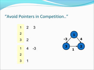
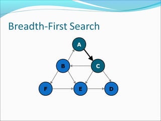
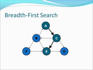
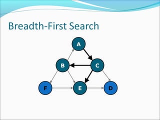
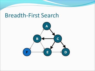
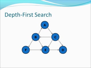
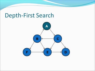
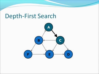
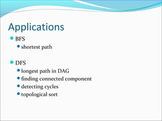
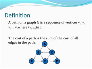
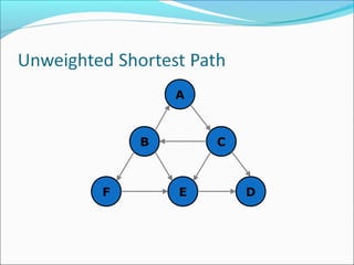
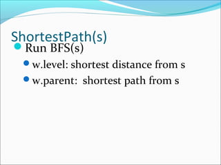
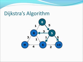
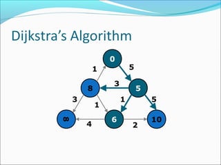
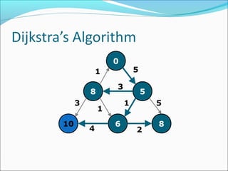
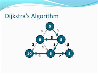
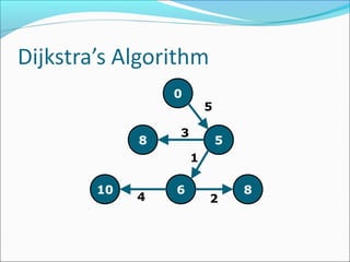
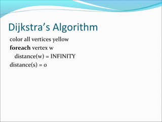
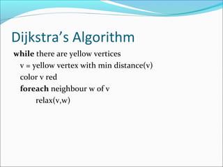
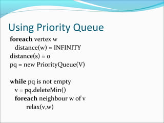
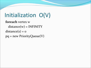
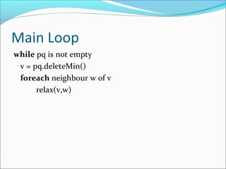
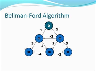
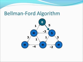
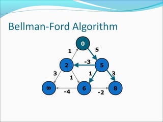
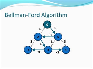
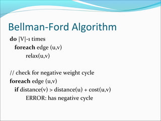
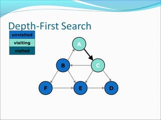
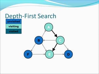
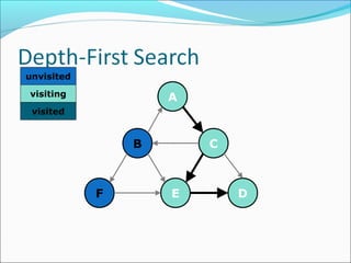
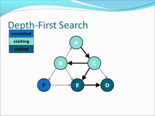
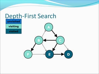
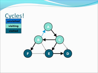
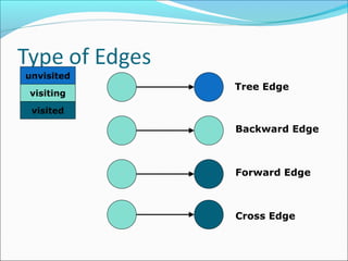
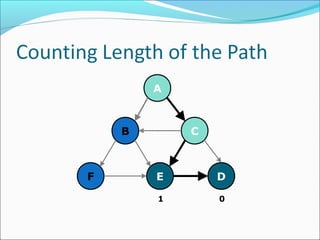
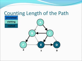
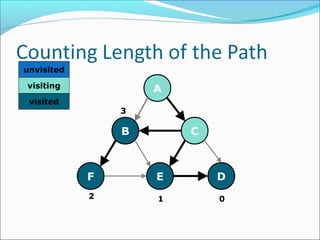
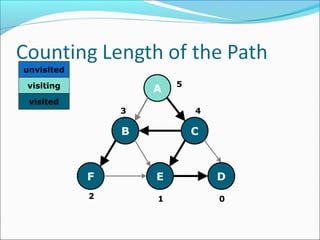
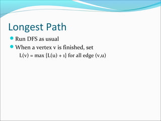
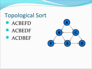
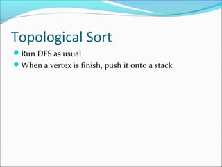
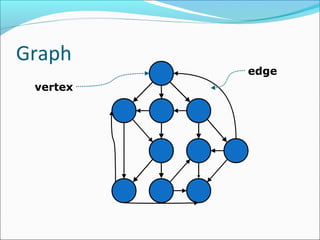
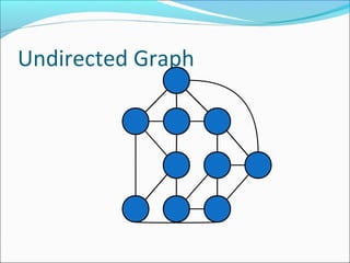
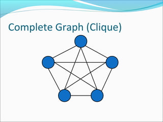
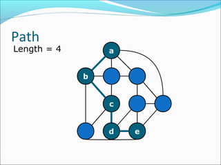
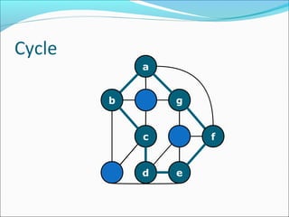
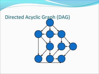
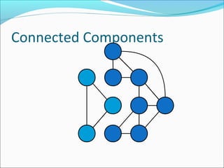
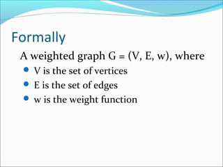
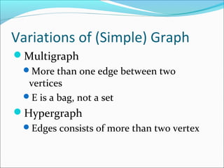
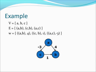
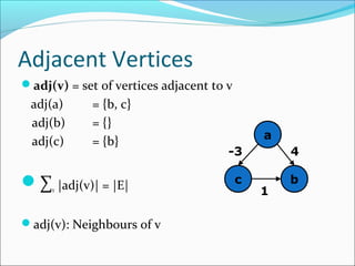
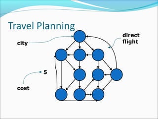
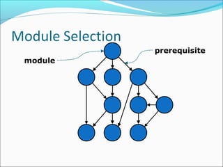
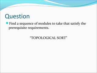
The document discusses using graphs to model real-world problems and algorithms for solving graph problems. It introduces basic graph terminology like vertices, edges, adjacency matrix/list representations. It then summarizes algorithms for finding shortest paths like Dijkstra's and Bellman-Ford. It also discusses using depth-first search to solve problems like detecting cycles, topological sorting of vertices, and calculating longest paths in directed acyclic graphs.

1. In science one tries to tell people, in such a way
as to be understood by everyone, something
that no one ever knew before.
But in poetry, it's the exact opposite.
Paul Dirac

2. Graph
vertex
edge

3. Weighted Graph
5
3
-2
5
1
0

4. Undirected Graph

5. Complete Graph (Clique)

6. Path
a
c
d e
b
Length = 4

7. Cycle
a
c
g
d e
b
f

8. Directed Acyclic Graph (DAG)

9. Degree

10. In-Degree Out-Degree

11. Disconnected Graph

12. Connected Components

13. Formally
A weighted graph G = (V, E, w), where
 V is the set of vertices
 E is the set of edges
 w is the weight function

14. Variations of (Simple) Graph
Multigraph
More than one edge between two
vertices
E is a bag, not a set
Hypergraph
Edges consists of more than two vertex

15. Example
V = { a, b, c }
E = { (a,b), (c,b), (a,c) }
w = { ((a,b), 4), ((c, b), 1), ((a,c),-3) }
a
bc
4
1
-3

16. Adjacent Vertices
adj(v) = set of vertices adjacent to v
adj(a) = {b, c}
adj(b) = {}
adj(c) = {b}
∑v |adj(v)| = |E|
adj(v): Neighbours of v
a
bc
4
1
-3

18. city
direct
flight
5
cost

19. QuestionWhat is the shortest way to travel between A and
B?
“SHORTEST PATH PROBLEM”
How to mimimize the cost of visiting n cities such
that we visit each city exactly once, and finishing
at the city where we start from?
“TRAVELING SALESMAN PROBLEM”

20. computer
network
link

21. Question
What is the shortest route to send a packet from A to
B?
“SHORTEST PATH PROBLEM”

22. web page
web link

23. module
prerequisite

24. Question
Find a sequence of modules to take that satisfy the
prerequisite requirements.
“TOPOLOGICAL SORT”

25. Other Applications
Biology
VLSI Layout
Vehicle Routing
Job Scheduling
Facility Location
:
:

27. Adjacency Matrix
double vertex[][];
1
23
4
1
-31 2 3
1 ∞ 4 -3
2 ∞ ∞ ∞
3 ∞ 1 ∞

28. Adjacency List
EdgeList vertex[];
1
23
4
1
-3
1
2
3
3 -3 2 4
2 1
neighbour cost

29. “Avoid Pointers in Competition..”
1
23
4
1
-3
1 2 3
2
3 2
1 4 -3
2
3 1

31. A
C
D
B
EF

32. A
C
D
B
EF

33. A
C
D
B
EF

34. A
C
D
B
EF

35. A
C
D
B
EF

36. A
C
D
B
EF

37. A
C
D
B
EF

38. A
C
D
B
EF

39. 0
1
2
2
23

40. Level-Order on Treeif T is empty return
Q = new Queue
Q.enq(T)
while Q is not empty
curr = Q.deq()
print curr.element
if T.left is not empty
Q.enq(curr.left)
if curr.right is not empty
Q.enq(curr.right)
1
4 5
3
6
9 08
2
7

41. Calculating LevelQ = new Queue
Q.enq (v)
v.level = 0
while Q is not empty
curr = Q.deq()
if curr is not visited
mark curr as visited
foreach w in adj(curr)
if w is not visited
w.level = curr.level + 1
Q.enq(w)
A
C
D
B
EF

42. Search All Vertices
Search(G)
foreach vertex v
mark v as unvisited
foreach vertex v
if v is not visited
BFS(v)

44. A
C
D
B
EF

45. A
C
D
B
EF

46. A
C
D
B
EF

48. Applications
BFS
shortest path
DFS
longest path in DAG
finding connected component
detecting cycles
topological sort

49. Definition
A path on a graph G is a sequence of vertices v0, v1,
v2, .. vnwhere (vi,vi+1)∈E
The cost of a path is the sum of the cost of all
edges in the path. A
C
D
B
EF

50. A
C
D
B
EF

51. ShortestPath(s)
Run BFS(s)
w.level: shortest distance from s
w.parent: shortest path from s

52. A
C
D
B
EF
5
51
2
3
1
3
1
4

53. BFS(s) does not work
Must keep track of smallest distance so far.
If we found a new, shorter path, update the distance.

54. 10
6
2
8
s w
v

55. Definition
distance(v) : shortest distance so far from s to v
parent(v) : previous node on the shortest path so far
from s to v
cost(u, v) : the cost of edge from u to v

56. 10
6
2
8
s w
v
distance(w) = 8
cost(v,w) = 2
parent(w) = v

57. A
C
D
B
EF
5
51
2
3
1
3
1
4

58. 0
8
8
8
8
8
5
51
2
3
1
3
1
4

59. 0
5
8
8
8
8
5
51
2
3
1
3
1
4

60. 0
5
8
8
8
8
5
51
2
3
1
3
1
4

61. 0
5
10
8
6
8
5
51
2
3
1
3
1
4

62. 0
5
10
8
6
8
5
51
2
3
1
3
1
4

63. 0
5
8
8
610
5
51
2
3
1
3
1
4

64. 0
5
8
8
610
5
51
2
3
1
3
1
4

65. 0
5
8
8
610
5
51
2
3
1
3
1
4

66. 0
5
8
8
610
5
51
2
3
1
3
1
4

67. 0
5
8
8
610
5
1
2
3
4

68. Dijkstra’s Algorithm
color all vertices yellow
foreach vertex w
distance(w) = INFINITY
distance(s) = 0

69. Dijkstra’s Algorithm
while there are yellow vertices
v = yellow vertex with min distance(v)
color v red
foreach neighbour w of v
relax(v,w)

70. Using Priority Queue
foreach vertex w
distance(w) = INFINITY
distance(s) = 0
pq = new PriorityQueue(V)
while pq is not empty
v = pq.deleteMin()
foreach neighbour w of v
relax(v,w)

71. Initialization O(V)
foreach vertex w
distance(w) = INFINITY
distance(s) = 0
pq = new PriorityQueue(V)

72. Main Loop
while pq is not empty
v = pq.deleteMin()
foreach neighbour w of v
relax(v,w)

73. 0
8
8
8
8
8
5
31
-2
-3
1
3
1
-4

74. 0
5
8
8
8
8
5
31
-2
-3
1
3
1
-4

75. 0
5
8
2
6
8
5
31
-2
-3
1
3
1
-4

76. 0
5
4
2
32
5
31
-2
-3
1
3
1
-4

77. 0
5
1
2
3-1
5
31
-2
-3
1
3
1
-4

78. Bellman-Ford Algorithm
do |V|-1 times
foreach edge (u,v)
relax(u,v)
// check for negative weight cycle
foreach edge (u,v)
if distance(v) > distance(u) + cost(u,v)
ERROR: has negative cycle

80. Idea: Use DFS
Denote vertex as “visited”, “unvisited” and “visiting”
Mark a vertex as “visited” = vertex is finished

81. A
C
D
B
EF
unvisited
visiting
visited

82. A
C
D
B
EF
unvisited
visiting
visited

83. A
C
D
B
EF
unvisited
visiting
visited

84. A
C
D
B
EF
unvisited
visiting
visited

85. A
C
D
B
EF
unvisited
visiting
visited

86. A
C
D
B
EF
unvisited
visiting
visited

87. A
C
D
B
EF
unvisited
visiting
visited

88. A
C
D
B
EF
unvisited
visiting
visited

89. A
C
D
B
EF
unvisited
visiting
visited

90. unvisited
visiting
visited
Tree Edge
Backward Edge
Forward Edge
Cross Edge

91. (in a DAG)

92. A
C
D
B
EF
1 0

93. A
C
D
B
EF
unvisited
visiting
visited
1 02

94. A
C
D
B
EF
unvisited
visiting
visited
1 0
3
2

95. A
C
D
B
EF
unvisited
visiting
visited
1 0
3 4
5
2

96. Longest Path
Run DFS as usual
When a vertex v is finished, set
L(v) = max {L(u) + 1} for all edge (v,u)

98. Topological Sort
Goal: Order the vertices, such that if there is a path
from u to v, u appears before v in the output.

99. Topological Sort
 ACBEFD
 ACBEDF
 ACDBEF
A
C
D
B
EF

100. Topological Sort
Run DFS as usual
When a vertex is finish, push it onto a stack