Downloaded 14 times
![R
C
C
h
a
k
r
a
b
o
r
t
y
,
w
w
w
.
m
y
r
e
a
d
e
r
s
.
i
n
f
o
SC – GA - Introduction
[Ref : previous slide Enumerative search]
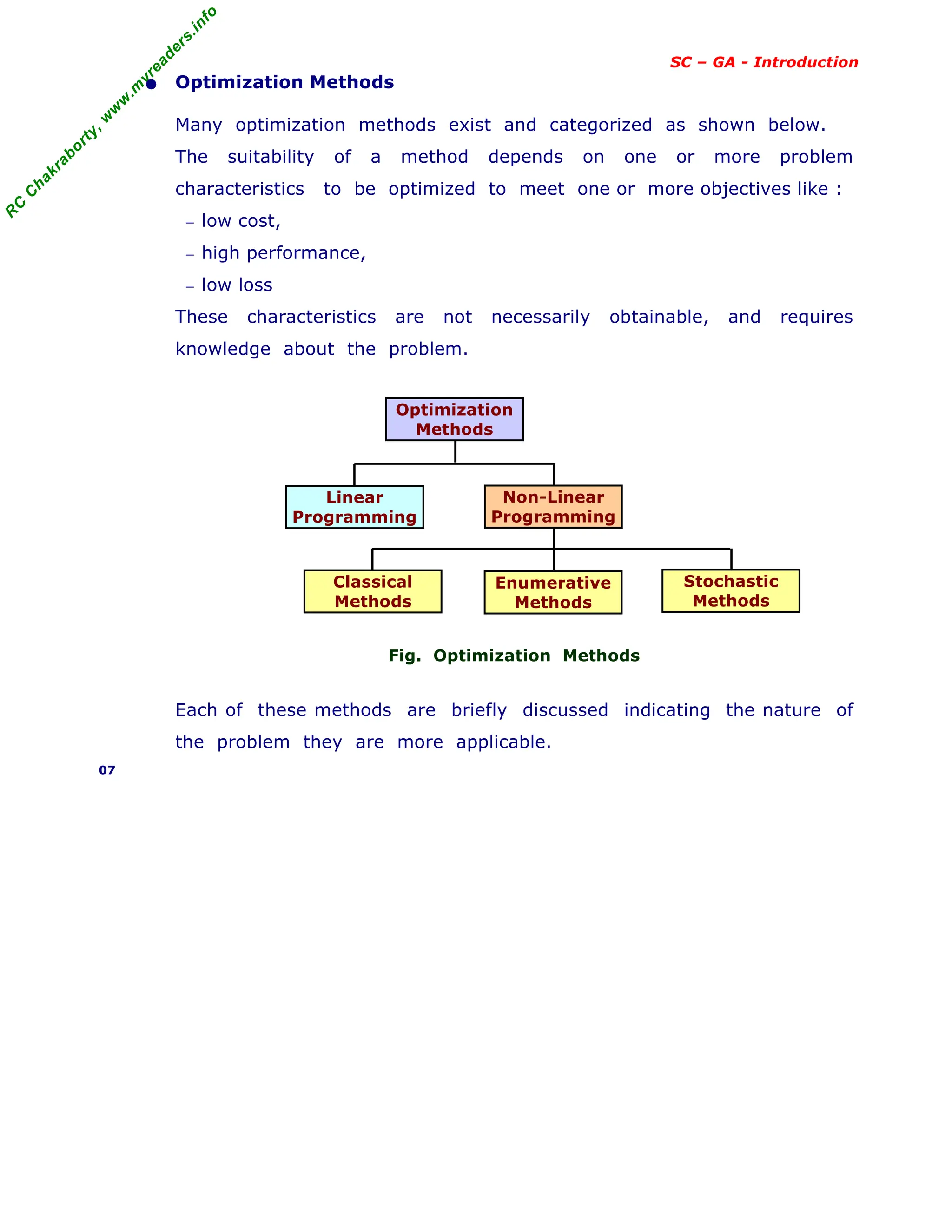
The Enumerative search techniques follows, the traditional search and
control strategies, in the domain of Artificial Intelligence.
− the search methods explore the search space "intelligently"; means
evaluating possibilities without investigating every single possibility.
− there are many control structures for search; the depth-first search
and breadth-first search are two common search strategies.
− the taxonomy of search algorithms in AI domain is given below.
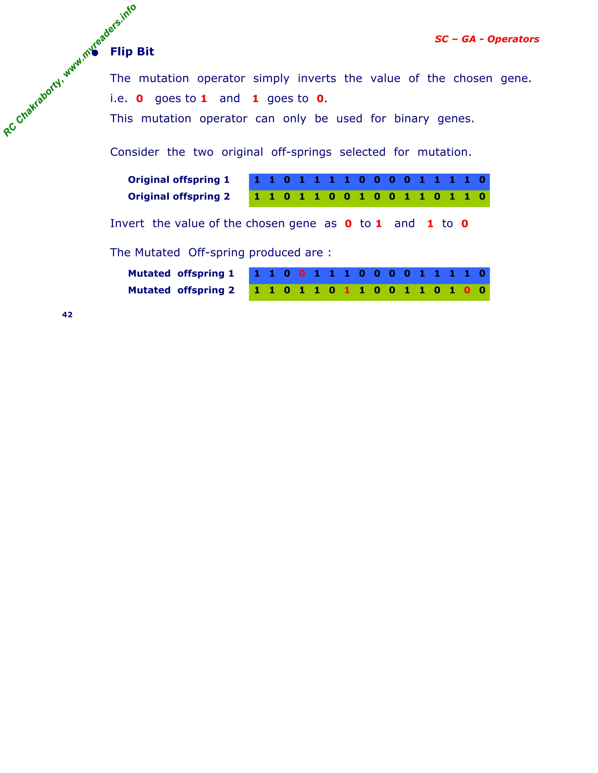
Fig. Enumerative Search Algorithms in AI Domain
13
User heuristics h(n)
No h(n) present
Priority Queue:
f(n)=h(n)+g(n
LIFO Stack
Gradually increase
fixed depth limit
Impose fixed
depth limit
Priority
Queue: g(n)
Priority
Queue: h(n)
FIFO
Enumerative Search
G (State, Operator, Cost)
Informed Search
Uninformed Search
Depth-First
Search
Breadth-First
Search
Cost-First
Search
Generate
-and-test
Hill
Climbing
Depth
Limited
Search
Iterative
Deepening
DFS
Problem
Reduction
Constraint
satisfaction
Mean-end-
analysis
Best first
search
A* Search AO* Search](https://image.slidesharecdn.com/08fundamentalsofgeneticalgorithms-240405042337-985f20df/75/Fundamentals-of-Genetic-Algorithms-Soft-Computing-13-2048.jpg)
![R
C
C
h
a
k
r
a
b
o
r
t
y
,
w
w
w
.
m
y
r
e
a
d
e
r
s
.
i
n
f
o
SC – GA - Introduction
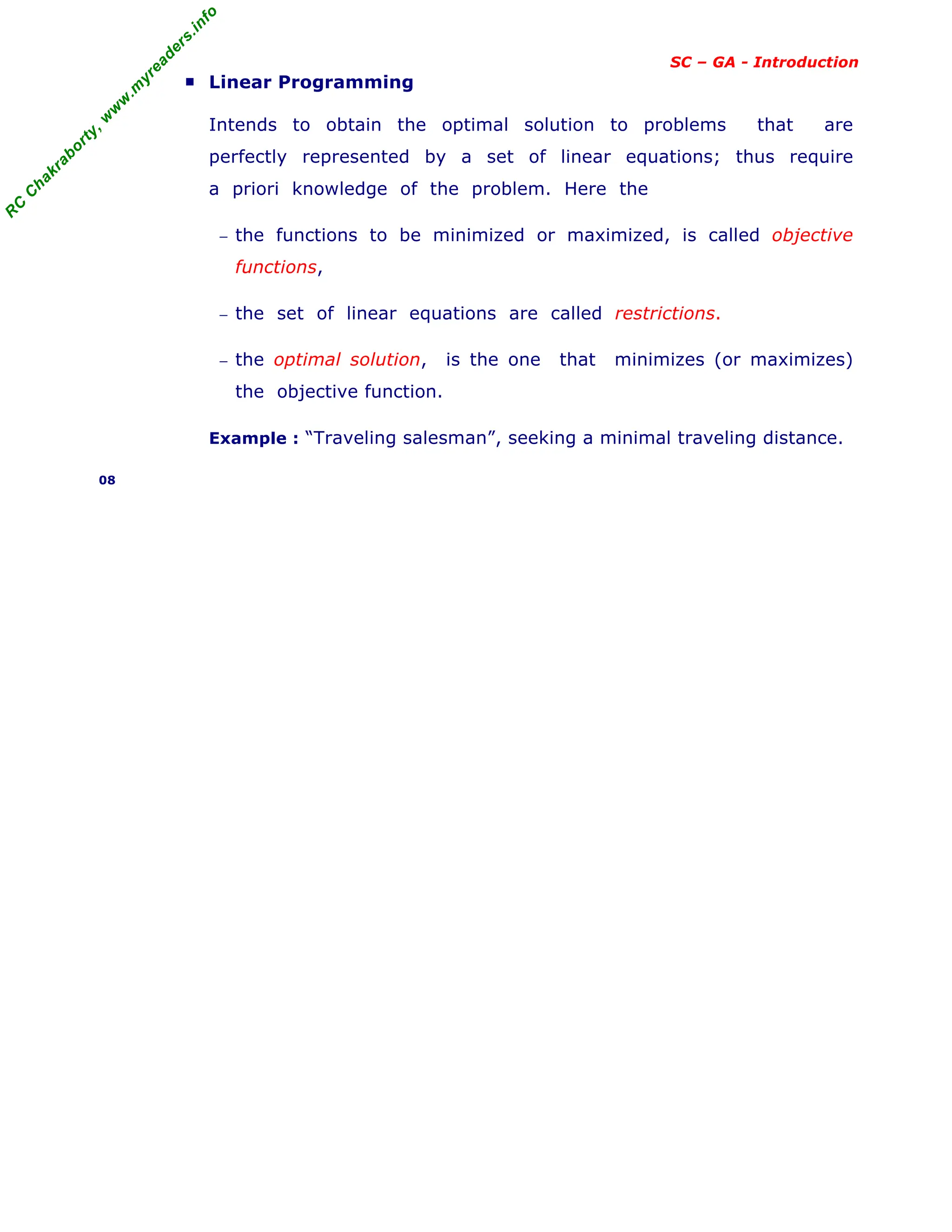
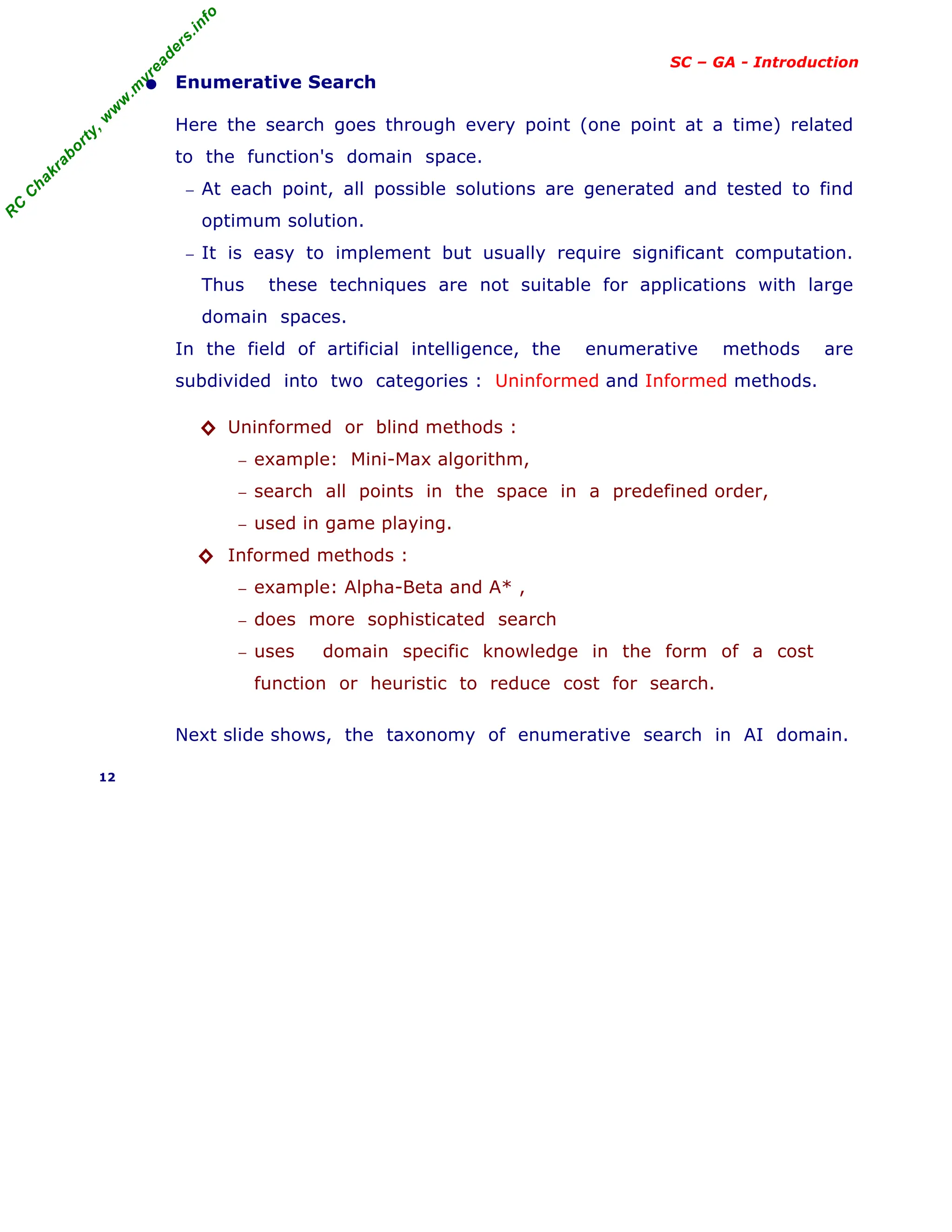
[ continued from previous slide - Biological background ]
Below shown, the general scheme of evolutionary process in genetic
along with pseudo-code.
Fig. General Scheme of Evolutionary process
Pseudo-Code
BEGIN
INITIALISE population with random candidate solution.
EVALUATE each candidate;
REPEAT UNTIL (termination condition ) is satisfied DO
1. SELECT parents;
2. RECOMBINE pairs of parents;
3. MUTATE the resulting offspring;
4. SELECT individuals or the next generation;
END.
19
Parents
Offspring
Population
Recombination
Mutation
Parents
Termination
Initialization
Survivor](https://image.slidesharecdn.com/08fundamentalsofgeneticalgorithms-240405042337-985f20df/75/Fundamentals-of-Genetic-Algorithms-Soft-Computing-19-2048.jpg)
![R
C
C
h
a
k
r
a
b
o
r
t
y
,
w
w
w
.
m
y
r
e
a
d
e
r
s
.
i
n
f
o
SC – GA - Introduction
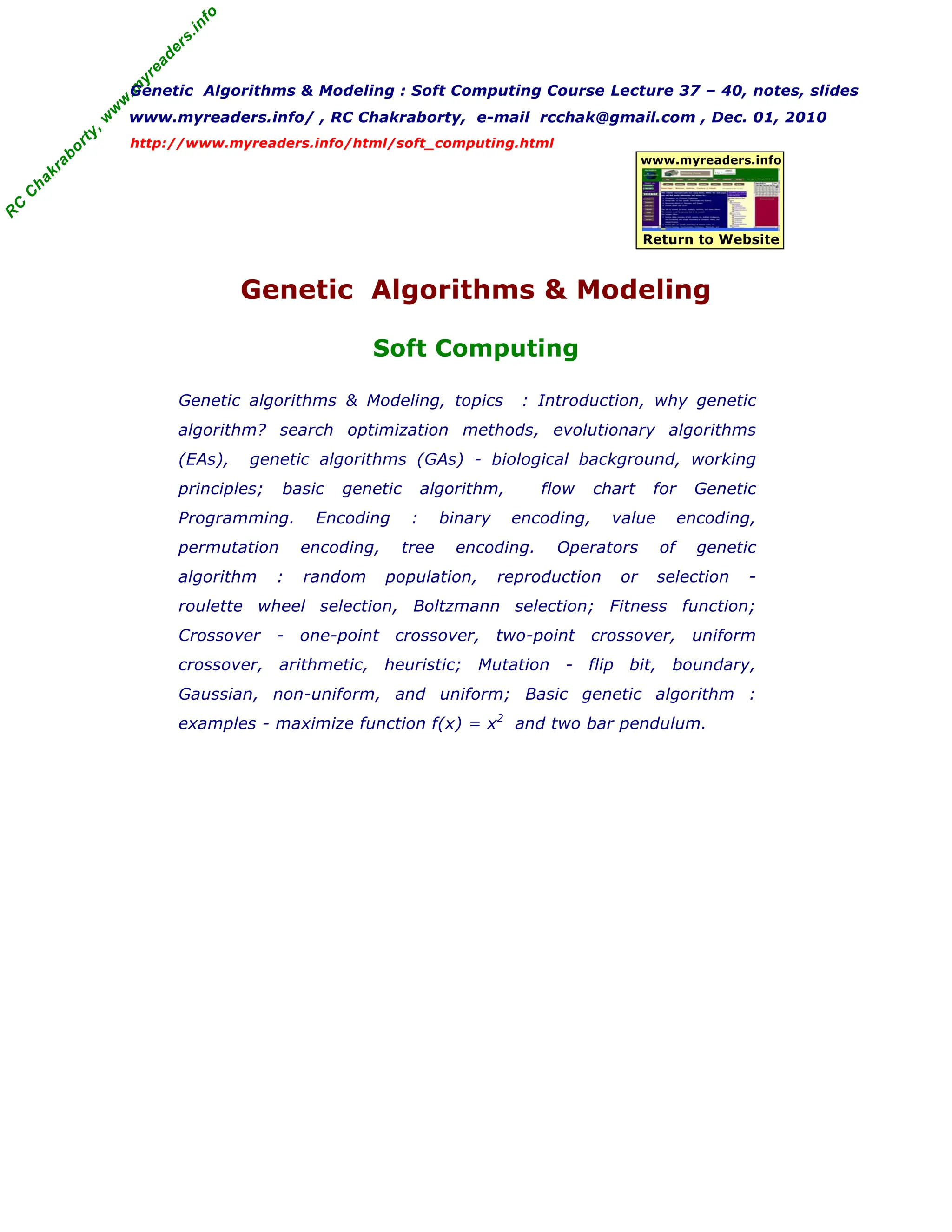
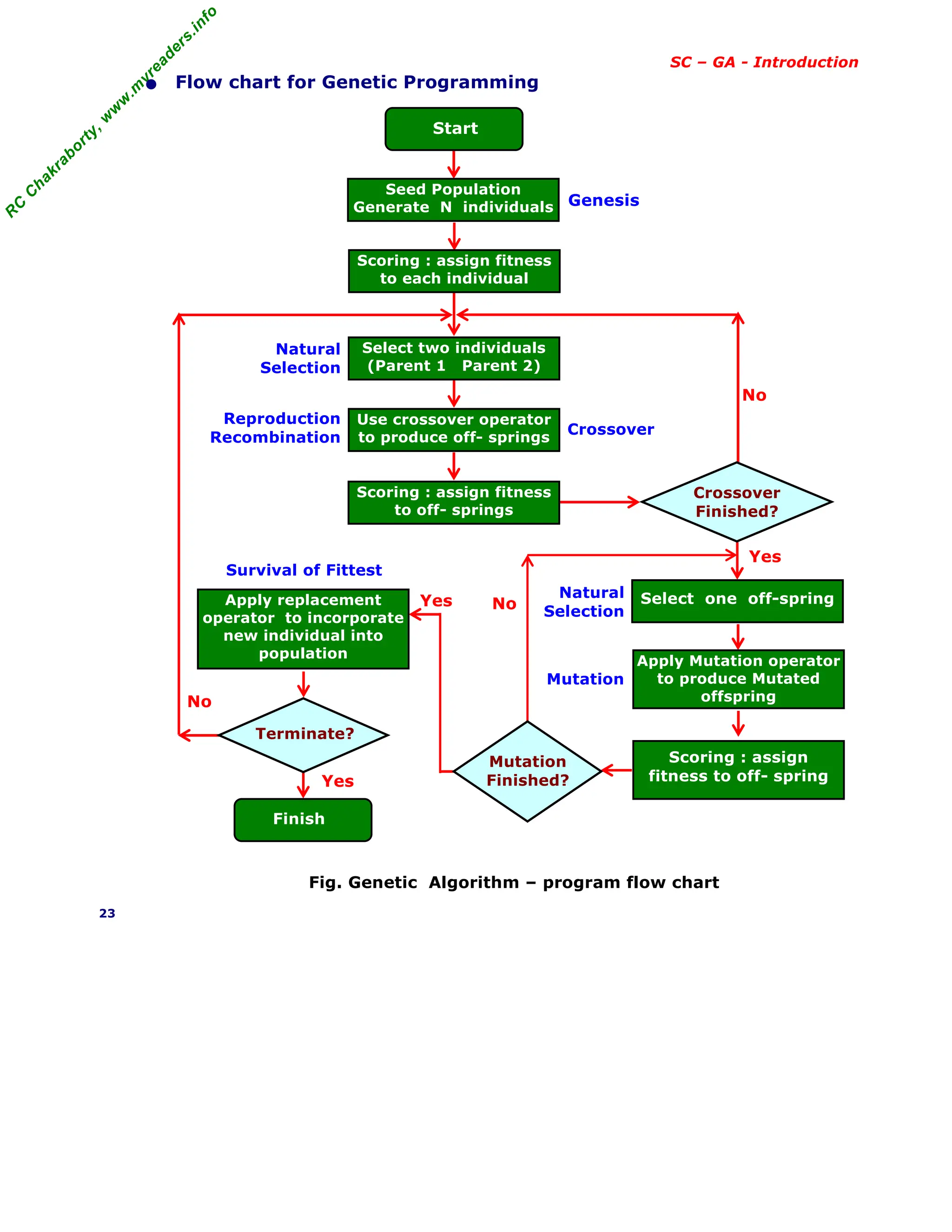
• Outline of the Basic Genetic Algorithm
1. [Start] Generate random population of n chromosomes (i.e. suitable
solutions for the problem).
2. [Fitness] Evaluate the fitness f(x) of each chromosome x in the
population.
3. [New population] Create a new population by repeating following
steps until the new population is complete.
(a) [Selection] Select two parent chromosomes from a population
according to their fitness (better the fitness, bigger the chance to
be selected)
(b) [Crossover] With a crossover probability, cross over the parents
to form new offspring (children). If no crossover was performed,
offspring is the exact copy of parents.
(c) [Mutation] With a mutation probability, mutate new offspring at
each locus (position in chromosome).
(d) [Accepting] Place new offspring in the new population
4. [Replace] Use new generated population for a further run of the
algorithm
5. [Test] If the end condition is satisfied, stop, and return the best
solution in current population
6. [Loop] Go to step 2
Note : The genetic algorithm's performance is largely influenced by two
operators called crossover and mutation. These two operators are the
most important parts of GA.
22](https://image.slidesharecdn.com/08fundamentalsofgeneticalgorithms-240405042337-985f20df/75/Fundamentals-of-Genetic-Algorithms-Soft-Computing-22-2048.jpg)
![R
C
C
h
a
k
r
a
b
o
r
t
y
,
w
w
w
.
m
y
r
e
a
d
e
r
s
.
i
n
f
o
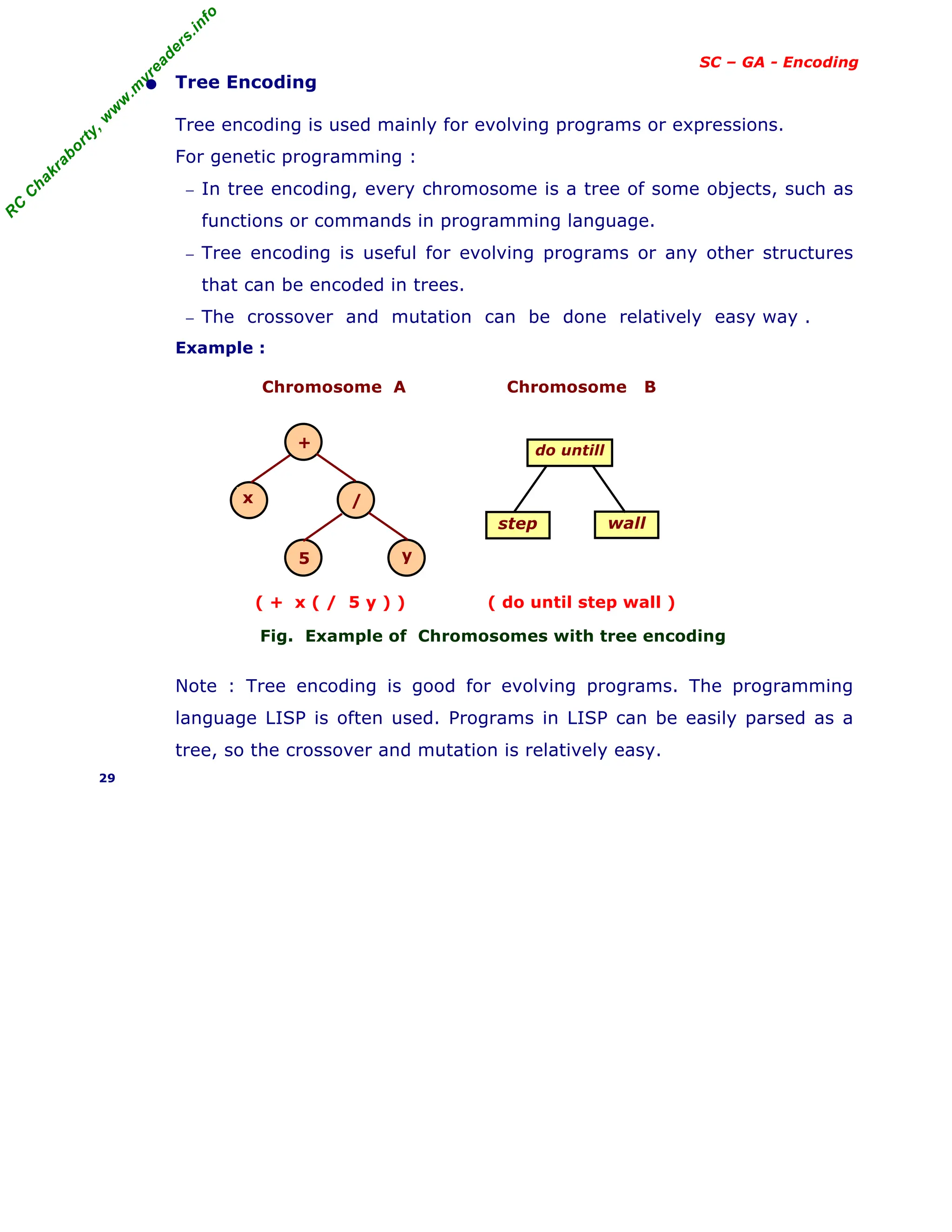
SC – GA - Encoding
[ continued binary encoding ]
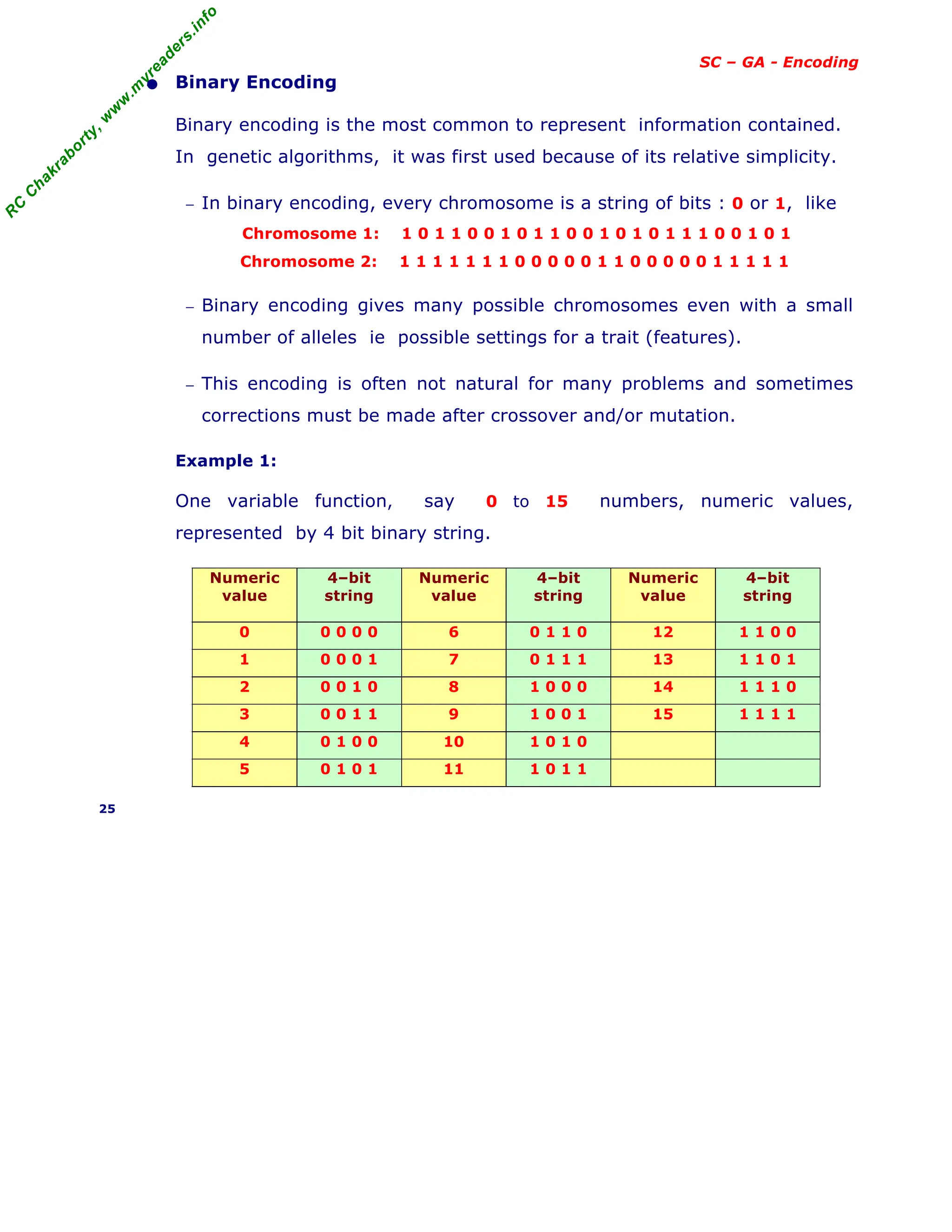
Example 2 :
Two variable function represented by 4 bit string for each variable.
Let two variables X1 , X2 as (1011 0110) .
Every variable will have both upper and lower limits as ≤ ≤
Because 4-bit string can represent integers from 0 to 15,
so (0000 0000) and (1111 1111) represent the points for X1 , X2 as
( , ) and ( , ) respectively.
Thus, an n-bit string can represent integers from
0 to 2n
-1, i.e. 2n
integers.
Binary Coding Equivalent integer Decoded binary substring
1 0 1 0
0 x 2
0
= 0
1 x 2
1
= 2
0 x 2
2
= 0
1 x 2
3
= 8
10
Let Xi is coded as a substring
Si of length ni. Then decoded
binary substring Si is as
where Si can be 0 or 1 and the
string S is represented as
Sn-1 . . . . S3 S2 S1 S0
Example : Decoding value
Consider a 4-bit string (0111),
− the decoded value is equal to
23
x 0 + 22
x 1 + 21
x 1 + 20
x 1 = 7
− Knowing and corresponding to (0000) and (1111) ,
the equivalent value for any 4-bit string can be obtained as
( − )
Xi = + --------------- x (decoded value of string)
( 2ni
− 1 )
− For e.g. a variable Xi ; let = 2 , and = 17, find what value the
4-bit string Xi = (1010) would represent. First get decoded value for
Si = 1010 = 23
x 1 + 22
x 0 + 21
x 1 + 20
x 0 = 10 then
(17 -2)
Xi = 2 + ----------- x 10 = 12
(24
- 1)
The accuracy obtained with a 4-bit code is 1/16 of search space.
By increasing the string length by 1-bit , accuracy increases to 1/32.
26
X
L
i
Xi
X
U
i
X
L
1 X
L
2
X
U
2
X
U
1
2 10 Remainder
2 5 0
2 2 1
1 0
Σ
k=0
K=ni - 1
2
k
Sk
X
L
i X
U
i
X
L
i
X
U
i
X
L
i
X
L
i X
U
i](https://image.slidesharecdn.com/08fundamentalsofgeneticalgorithms-240405042337-985f20df/75/Fundamentals-of-Genetic-Algorithms-Soft-Computing-26-2048.jpg)
![R
C
C
h
a
k
r
a
b
o
r
t
y
,
w
w
w
.
m
y
r
e
a
d
e
r
s
.
i
n
f
o
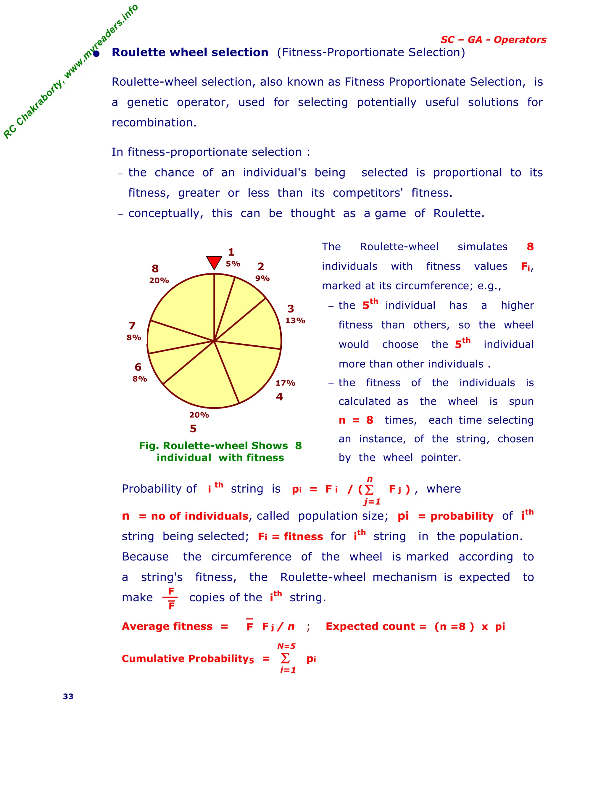
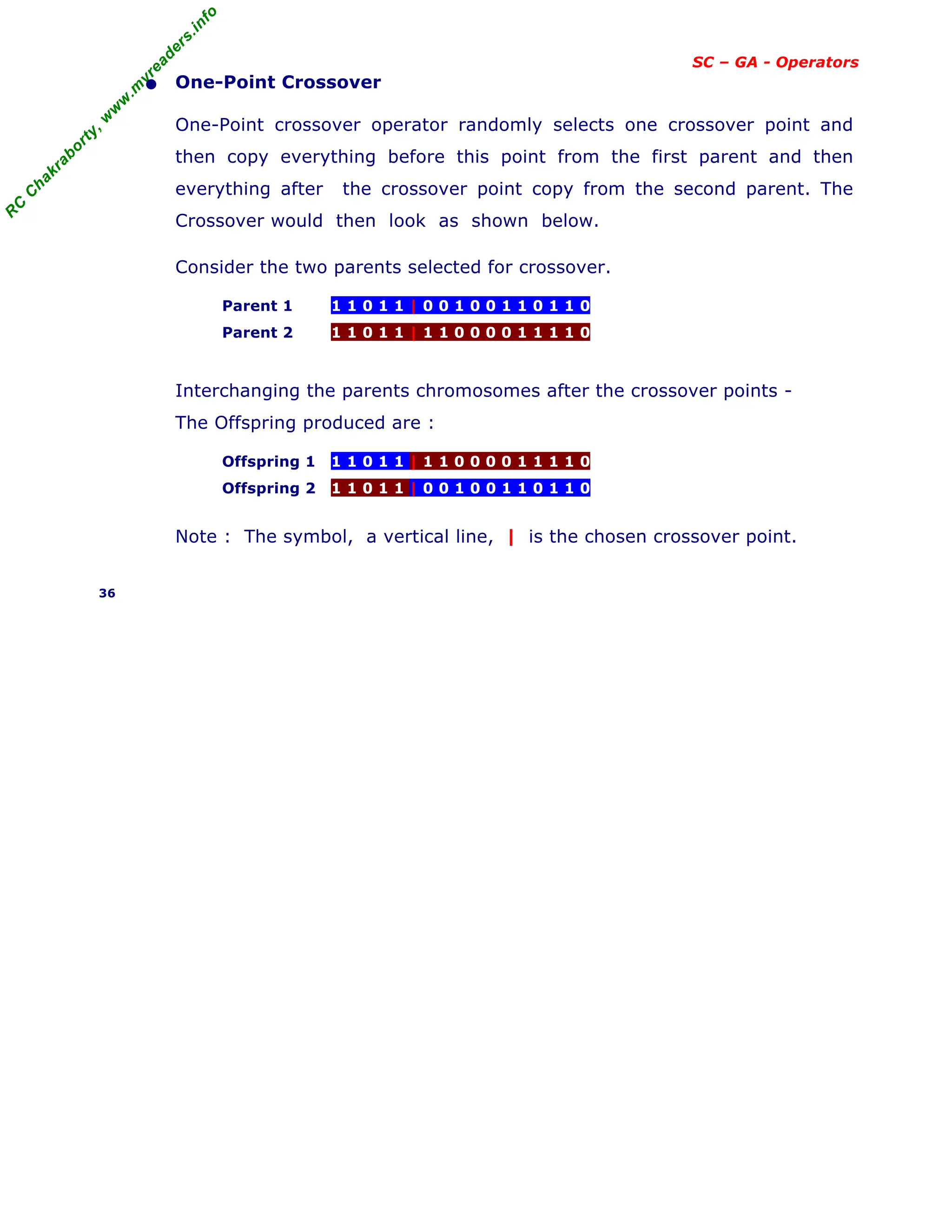
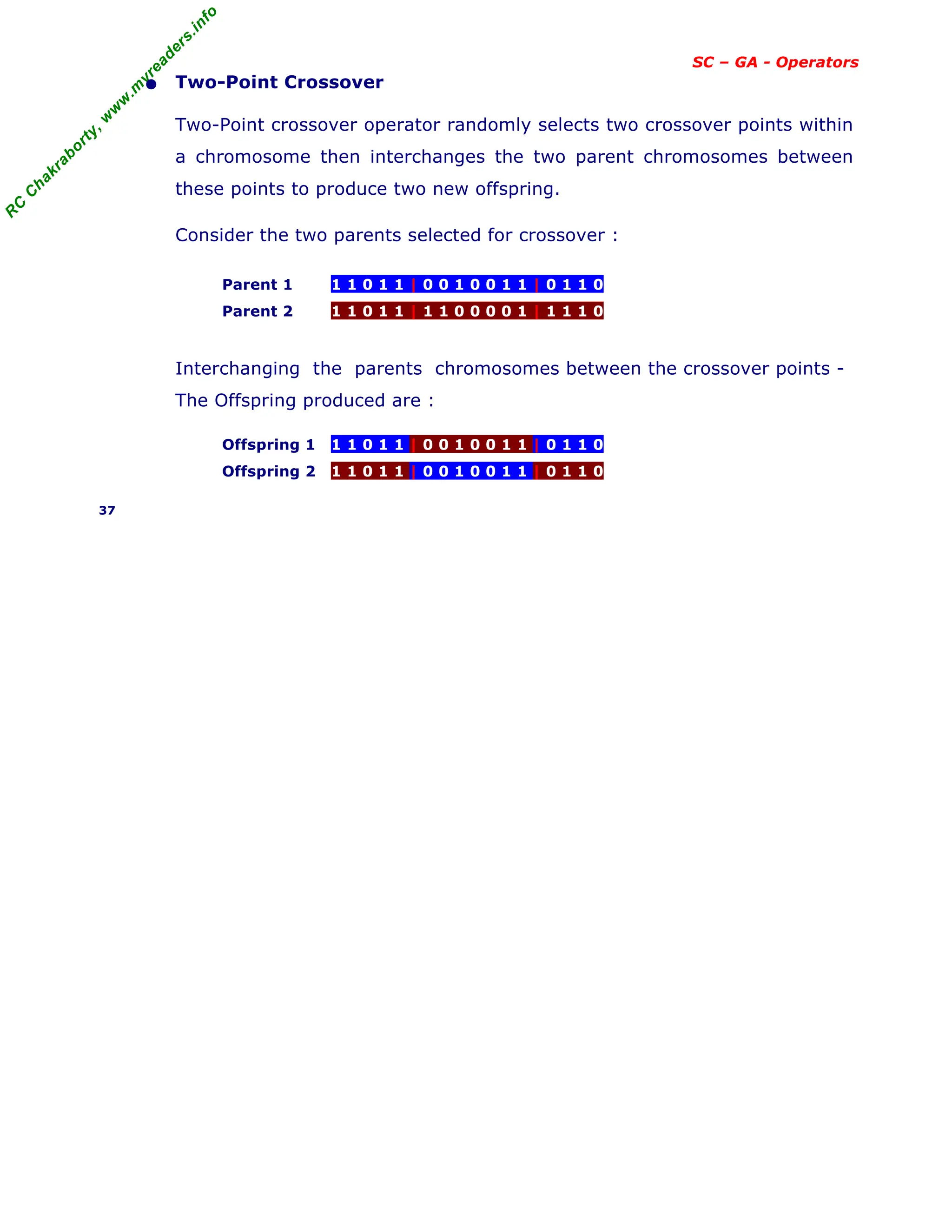
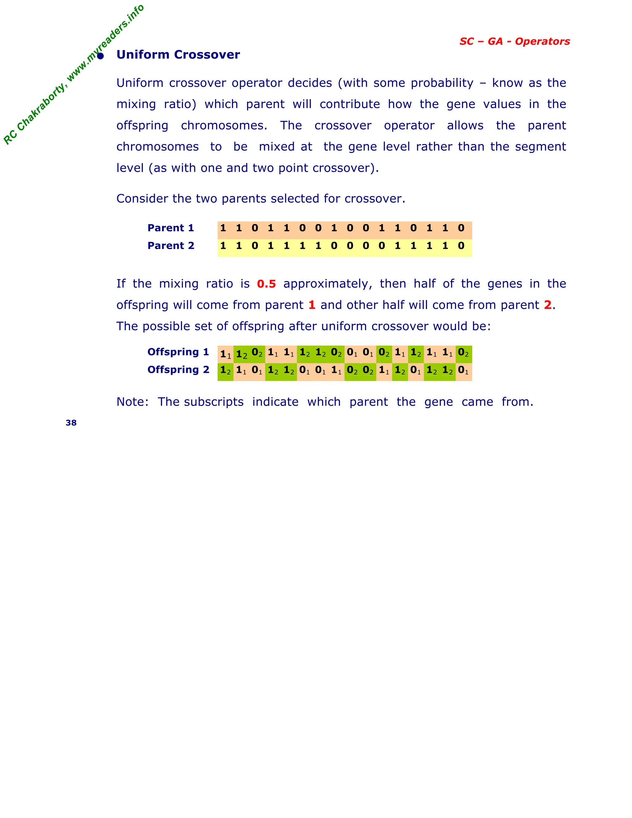
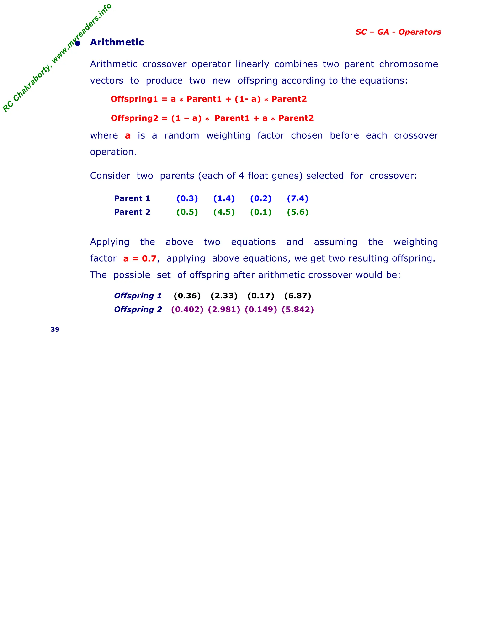
SC – GA - Operators
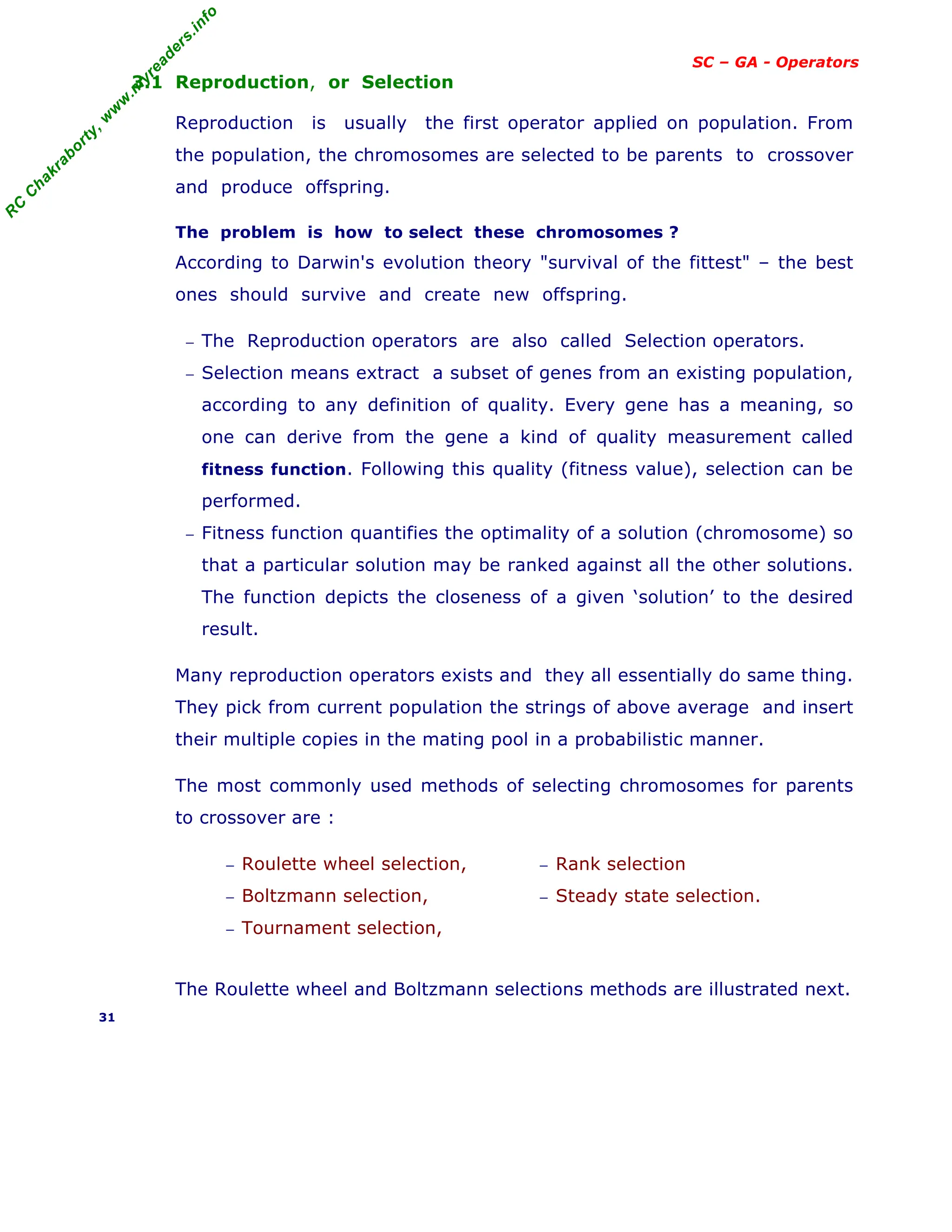
• Example of Selection
Evolutionary Algorithms is to maximize the function f(x) = x2
with x in
the integer interval [0 , 31], i.e., x = 0, 1, . . . 30, 31.
1. The first step is encoding of chromosomes; use binary representation
for integers; 5-bits are used to represent integers up to 31.
2. Assume that the population size is 4.
3. Generate initial population at random. They are chromosomes or
genotypes; e.g., 01101, 11000, 01000, 10011.
4. Calculate fitness value for each individual.
(a) Decode the individual into an integer (called phenotypes),
01101 → 13; 11000 → 24; 01000 → 8; 10011 → 19;
(b) Evaluate the fitness according to f(x) = x2
,
13 → 169; 24 → 576; 8 → 64; 19 → 361.
5. Select parents (two individuals) for crossover based on their fitness
in pi. Out of many methods for selecting the best chromosomes, if
roulette-wheel selection is used, then the probability of the i
th
string
in the population is pi = F i / ( F j ) , where
F i is fitness for the string i in the population, expressed as f(x)
pi is probability of the string i being selected,
n is no of individuals in the population, is population size, n=4
n * pi is expected count
String No Initial
Population
X value Fitness Fi
f(x) = x2
p i Expected count
N * Prob i
1 0 1 1 0 1 13 169 0.14 0.58
2 1 1 0 0 0 24 576 0.49 1.97
3 0 1 0 0 0 8 64 0.06 0.22
4 1 0 0 1 1 19 361 0.31 1.23
Sum 1170 1.00 4.00
Average 293 0.25 1.00
Max 576 0.49 1.97
The string no 2 has maximum chance of selection.
32
Σ
j=1
n](https://image.slidesharecdn.com/08fundamentalsofgeneticalgorithms-240405042337-985f20df/75/Fundamentals-of-Genetic-Algorithms-Soft-Computing-32-2048.jpg)
![R
C
C
h
a
k
r
a
b
o
r
t
y
,
w
w
w
.
m
y
r
e
a
d
e
r
s
.
i
n
f
o
SC – GA - Examples
[ continued from previous slide ]
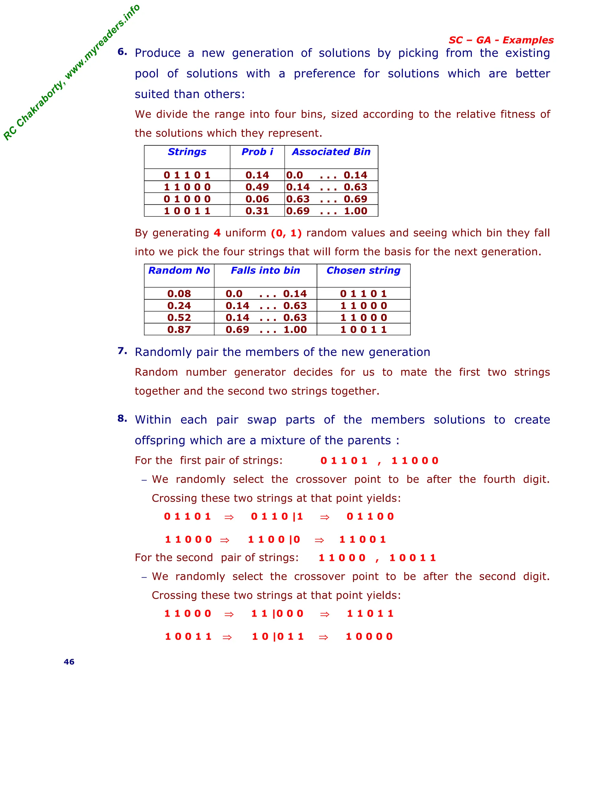
Genetic Algorithm approach to problem - Maximize the function f(x) = x2
1. Devise a means to represent a solution to the problem :
Assume, we represent x with five-digit unsigned binary integers.
2. Devise a heuristic for evaluating the fitness of any particular solution :
The function f(x) is simple, so it is easy to use the f(x) value itself to rate
the fitness of a solution; else we might have considered a more simpler
heuristic that would more or less serve the same purpose.
3. Coding - Binary and the String length :
GAs often process binary representations of solutions. This works well,
because crossover and mutation can be clearly defined for binary solutions.
A Binary string of length 5 can represents 32 numbers (0 to 31).
4. Randomly generate a set of solutions :
Here, considered a population of four solutions. However, larger populations
are used in real applications to explore a larger part of the search. Assume,
four randomly generated solutions as : 01101, 11000, 01000, 10011.
These are chromosomes or genotypes.
5. Evaluate the fitness of each member of the population :
The calculated fitness values for each individual are -
(a) Decode the individual into an integer (called phenotypes),
01101 → 13; 11000 → 24; 01000 → 8; 10011 → 19;
(b) Evaluate the fitness according to f(x) = x 2
,
13 → 169; 24 → 576; 8 → 64; 19 → 361.
(c) Expected count = N * Prob i , where N is the number of
individuals in the population called population size, here N = 4.
Thus the evaluation of the initial population summarized in table below .
String No
i
Initial
Population
(chromosome)
X value
(Pheno
types)
Fitness
f(x) = x2
Prob i
(fraction
of total)
Expected count
N * Prob i
1 0 1 1 0 1 13 169 0.14 0.58
2 1 1 0 0 0 24 576 0.49 1.97
3 0 1 0 0 0 8 64 0.06 0.22
4 1 0 0 1 1 19 361 0.31 1.23
Total (sum) 1170 1.00 4.00
Average 293 0.25 1.00
Max 576 0.49 1.97
Thus, the string no 2 has maximum chance of selection.
45](https://image.slidesharecdn.com/08fundamentalsofgeneticalgorithms-240405042337-985f20df/75/Fundamentals-of-Genetic-Algorithms-Soft-Computing-45-2048.jpg)

![R
C
C
h
a
k
r
a
b
o
r
t
y
,
w
w
w
.
m
y
r
e
a
d
e
r
s
.
i
n
f
o
SC – GA - Examples
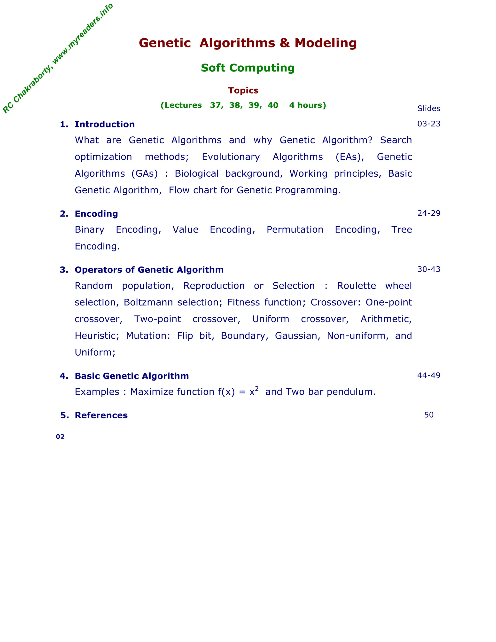
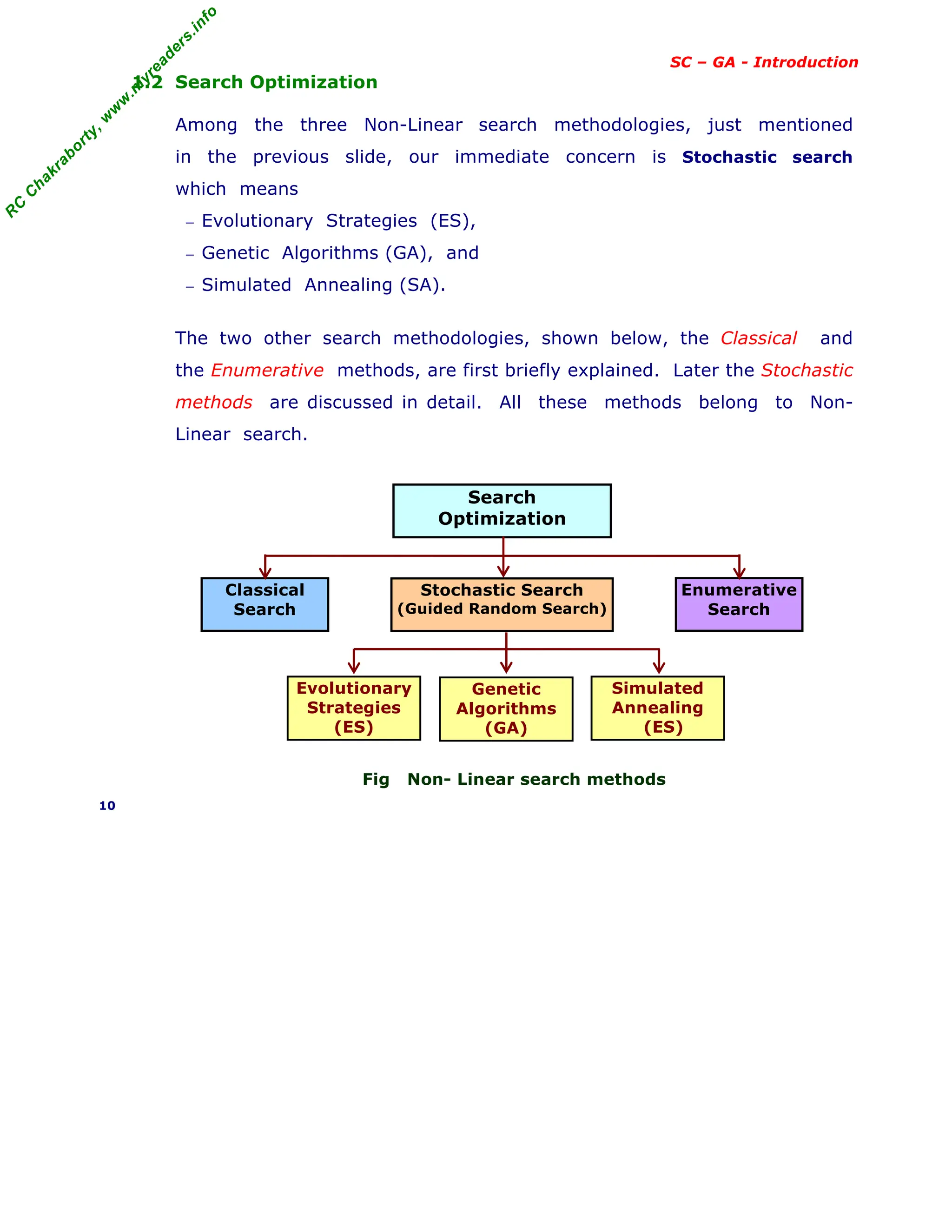
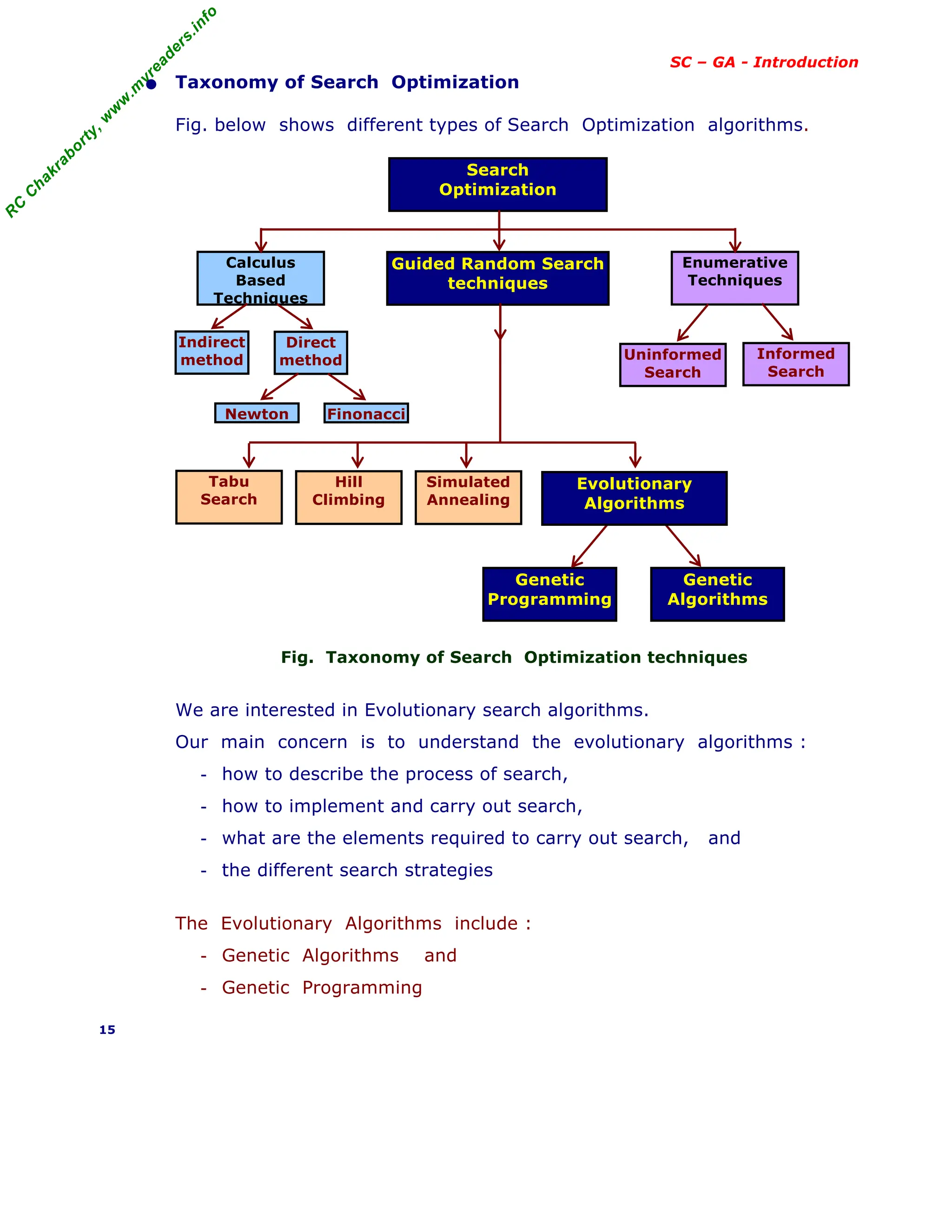
• Example 2 : Two bar pendulum
Two uniform bars are connected by pins at A and B and supported
at A. Let a horizontal force P acts at C.
Fig. Two bar pendulum
Given : Force P = 2, Length of bars ℓ1 = 2 ,
ℓ2 = 2, Bar weights W1= 2, W2 = 2 . angles = Xi
Find : Equilibrium configuration of the system if
fiction at all joints are neglected ?
Solution : Since there are two unknowns θ1 and
θ2 , we use 4 – bit binary for each unknown.
XU
- XL
90 - 0
Accuracy = ----------- = --------- = 60
24
- 1 15
Hence, the binary coding and the corresponding angles Xi are given as
XiU
- XiL
Xi = Xi
L
+ ----------- Si where Si is decoded Value of the i th
chromosome.
24
- 1
e.g. the 6th chromosome binary code (0 1 0 1) would have the corresponding
angle given by Si = 0 1 0 1 = 23
x 0 + 22
x 1 + 21
x 0 + 20
x 1 = 5
90 - 0
Xi = 0 + ----------- x 5 = 30
15
The binary coding and the angles are given in the table below.
S. No. Binary code
Si
Angle
Xi
S. No. Binary code
Si
Angle
Xi
1 0 0 0 0 0 9 1 0 0 0 48
2 0 0 0 1 6 10 1 0 0 1 54
3 0 0 1 0 12 11 1 0 1 0 60
4 0 0 1 1 18 12 1 0 1 1 66
5 0 1 0 0 24 13 1 1 0 0 72
6 0 1 0 1 30 14 1 1 0 1 78
7 0 1 1 0 36 15 1 1 1 0 84
8 0 1 1 1 42 16 1 1 1 1 90
Note : The total potential for two bar pendulum is written as
∏ = - P[(ℓ1 sinθ1 + ℓ2 sinθ2 )] - (W1 ℓ1 /2)cosθ1 - W2 [(ℓ2 /2) cosθ2 + ℓ1 cosθ1] (Eq.1)
Substituting the values for P, W1 , W2 , ℓ1 , ℓ2 all as 2 , we get ,
∏ (θ1 , θ2 ) = - 4 sinθ1 - 6 cosθ1 - 4 sinθ2 - 2 cosθ2 = function f (Eq. 2)
θ1 , θ2 lies between 0 and 90 both inclusive ie 0 ≤ θ1 , θ2 ≤ 90 (Eq. 3)
Equilibrium configuration is the one which makes ∏ a minimum .
Since the objective function is –ve , instead of minimizing the function f let us
maximize -f = f ’ . The maximum value of f ’ = 8 when θ1 and θ2 are zero.
Hence the fitness function F is given by F = – f – 7 = f ’ – 7 (Eq. 4)
48
W2
W1
y
A
θ2
θ1
ℓ2
B
C
P
ℓ1](https://image.slidesharecdn.com/08fundamentalsofgeneticalgorithms-240405042337-985f20df/75/Fundamentals-of-Genetic-Algorithms-Soft-Computing-48-2048.jpg)
![R
C
C
h
a
k
r
a
b
o
r
t
y
,
w
w
w
.
m
y
r
e
a
d
e
r
s
.
i
n
f
o
SC – GA - Examples
[ continued from previous slide ]
First randomly generate 8 population with 8 bit strings as shown in table below.
Population
No.
Population of 8 bit strings
(Randomly generated)
Corresponding Angles
(from table above)
θ1 , θ2
F = – f – 7
1 0 0 0 0 0 0 0 0 0 0 1
2 0 0 1 0 0 0 0 0 12 6 2.1
3 0 0 0 1 0 0 0 0 6 30 3.11
4 0 0 1 0 1 0 0 0 12 48 4.01
5 0 1 1 0 1 0 1 0 36 60 4.66
6 1 1 1 0 1 0 0 0 84 48 1.91
7 1 1 1 0 1 1 0 1 84 78 1.93
8 0 1 1 1 1 1 0 0 42 72 4.55
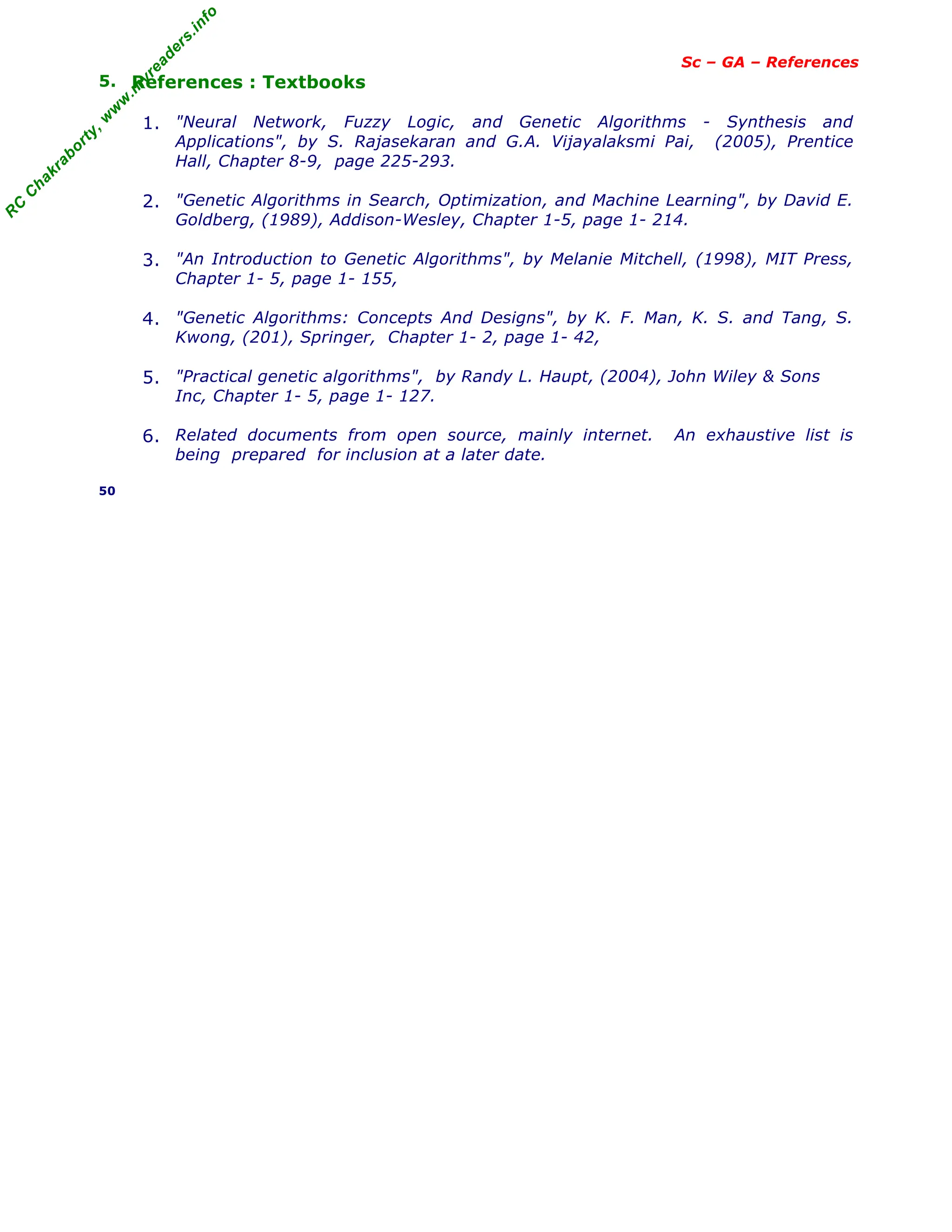
These angles and the corresponding to fitness function are shown below.
Fig. Fitness function F for various population
The above Table and the Fig. illustrates that :
− GA begins with a population of random strings.
− Then, each string is evaluated to find the fitness value.
− The population is then operated by three operators –
Reproduction , Crossover and Mutation, to create new population.
− The new population is further evaluated tested for termination.
− If the termination criteria are not met, the population is iteratively operated
by the three operators and evaluated until the termination criteria are met.
− One cycle of these operation and the subsequent evaluation procedure is
known as a Generation in GA terminology.
49
F=1
θ1=0
θ2=0
F=2.1
θ1=12
θ2=6
F=3.11
θ1=6
θ2=30
F=3.11
θ1=12
θ2=48
F=1.91
θ1=84
θ2=48
F=1.93
θ1=84
θ2=78
F=4.55
θ1=42
θ2=72
F=4.6
θ1=36
θ2=60](https://image.slidesharecdn.com/08fundamentalsofgeneticalgorithms-240405042337-985f20df/75/Fundamentals-of-Genetic-Algorithms-Soft-Computing-49-2048.jpg)

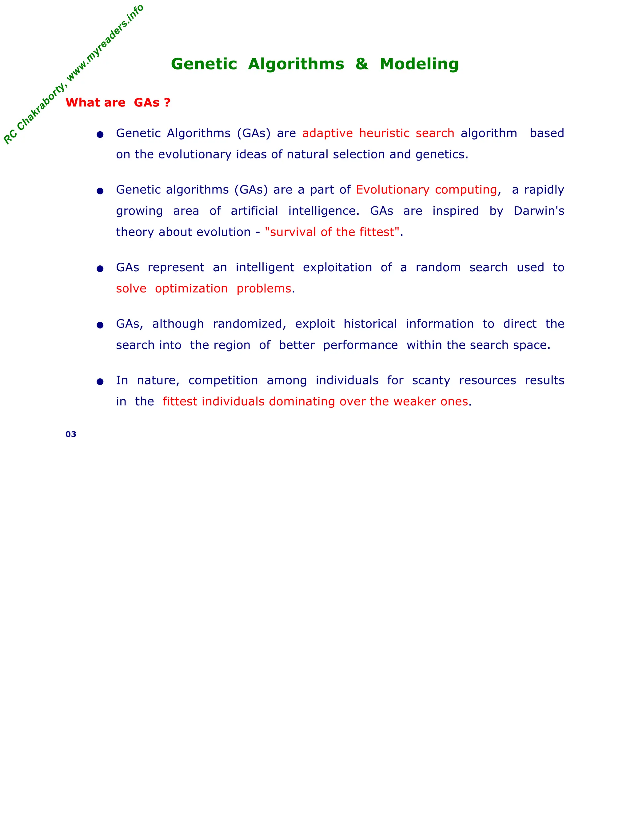
The document covers genetic algorithms (GAs) as adaptive heuristic search algorithms influenced by natural selection and genetics, detailing their function, encoding methods, and operational principles. It discusses the effectiveness of GAs in search optimization, their various types including evolutionary algorithms, and compares them to traditional optimization methods. Additionally, it emphasizes the practical applications and benefits of GAs in solving complex optimization problems.