The document discusses connected components and directed graphs, explaining how to determine if vertices are connected or if a graph is acyclic and connected (defining trees). It introduces algorithms such as BFS and DFS to check connectivity, and it details the process of topological sorting for directed acyclic graphs. Additionally, it covers concepts like indegree, outdegree, and their significance in representing task dependencies in directed graphs.

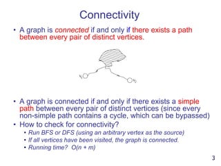
1. Connected Components,
Directed graphs,
Topological sort
Continuation of Graph
1

2. Application 1: Connectivity
D
E
A
C
F
B
G
K
H
L
N
M
O
R
Q
P
s
How do we tell if two vertices
are connected?
A connected to F?
A connected to L?
G =
2

3. Connectivity
• A graph is connected if and only if there exists a path
between every pair of distinct vertices.
• A graph is connected if and only if there exists a simple
path between every pair of distinct vertices (since every
non-simple path contains a cycle, which can be bypassed)
• How to check for connectivity?
• Run BFS or DFS (using an arbitrary vertex as the source)
• If all vertices have been visited, the graph is connected.
• Running time? O(n + m)
3

4. Connected Components
4

5. Subgraphs
5

6. Connected Components
• Formally stated:
• A connected component is a maximal connected subgraph of
a graph.
• The set of connected components is unique for a given graph.
6

7. Finding Connected Components
For each vertex
Call DFS
This will find
all vertices
connected
to “v” => one
connected component
Basic DFS algorithm.
If not visited
7

8. Time Complexity
• Running time for each i connected component
• Question:
• Can two connected components have the same edge?
• Can two connected components have the same vertex?
• So:
)( ii mnO 
 
i
i
i
i
i
ii mnOmnOmnO )()()(
8

9. Trees
• Tree arises in many computer science applications
• A graph G is a tree if and only if it is connected and acyclic
(Acyclic means it does not contain any simple cycles)
• The following statements are equivalent
• G is a tree
• G is acyclic and has exactly n-1 edges
• G is connected and has exactly n-1 edges
9

10. Tree as a (directed) Graph
15
6 18
3 8 30
16
Is it a graph?
Does it contain cycles?
(in other words, is it acyclic)
How many vertices?
How many edges?
10

11. Directed Graph
• A graph is directed if direction is assigned to each
edge. We call the directed edges arcs.
• An edge is denoted as an ordered pair (u, v)
• Recall: for an undirected graph
• An edge is denoted {u,v}, which actually corresponds to two
arcs (u,v) and (v,u)
11

12. Representations
• The adjacency matrix and adjacency list can be used
12

13. Directed Acyclic Graph
• A directed path is a sequence of vertices
(v0, v1, . . . , vk)
• Such that (vi, vi+1) is an arc
• A directed cycle is a directed path such that the first
and last vertices are the same.
• A directed graph is acyclic if it does not contain any
directed cycles
13

14. Indegree and Outdegree
• Since the edges are directed
• We can’t simply talk about Deg(v)
• Instead, we need to consider the arcs coming “in” and
going “out”
• Thus, we define terms
• Indegree(v)
• Outdegree(v)
14

15. Outdegree
• All of the arcs going “out” from v
• Simple to compute
• Scan through list Adj[v] and count the arcs
• What is the total outdegree? (m=#edges)
mv
v
vertex
)(outdegree
15

16. Indegree
• All of the arcs coming “in” to v
• Not as simple to compute as outdegree
• First, initialize indegree[v]=0 for each vertex v
• Scan through adj[v] list for each v
• For each vertex w seen, indegree[w]++;
• Running time: O(n+m)
• What is the total indegree?
mv
v
vertex
)(indegree
16

17. Indegree + Outdegree
• Each arc (u,v) contributes count 1 to the outdegree of
u and count 1 to the indegree of v.
mvv
v
 )(outdegree)(indegree
vertex
17

18. Example
0
1
2
3
4
5
6
7
8
9
Indeg(2)?
Indeg(8)?
Outdeg(0)?
Num of Edges?
Total OutDeg?
Total Indeg?
18

19. Directed Graphs Usage
• Directed graphs are often used to represent order-
dependent tasks
• That is we cannot start a task before another task finishes
• We can model this task dependent constraint using arcs
• An arc (i,j) means task j cannot start until task i is finished
• Clearly, for the system not to hang, the graph must be
acyclic.
i j
Task j cannot start
until task i is finished
19

20. Topological Sort
• Topological sort is an algorithm for a directed acyclic
graph
• It can be thought of as a way to linearly order the
vertices so that the linear order respects the ordering
relations implied by the arcs
0
1
2
3
4
5
6
7
8
9
For example:
0, 1, 2, 5, 9
0, 4, 5, 9
0, 6, 3, 7 ?
20

21. Topological Sort
• Idea:
• Starting point must have zero indegree!
• If it doesn’t exist, the graph would not be acyclic
1. A vertex with zero indegree is a task that can start
right away. So we can output it first in the linear
order
2. If a vertex i is output, then its outgoing arcs (i, j) are
no longer useful, since tasks j does not need to wait
for i anymore- so remove all i’s outgoing arcs
3. With vertex i removed, the new graph is still a
directed acyclic graph. So, repeat step 1-2 until no
vertex is left.
21

22. Topological Sort
Find all starting points
Reduce indegree(w)
Place new start
vertices on the Q
22

23. Example
0
1
2
3
4
5
6
7
8
9
0
1
2
3
4
5
6
7
8
9
2
6 1 4
7 5
8
5
3 2
8
9
9
0
1
2
3
4
5
6
7
8
9
0
1
2
1
1
2
1
1
2
2
Indegree
start
Q = { 0 }
OUTPUT: 0 23

24. Example
0
1
2
3
4
5
6
7
8
9
0
1
2
3
4
5
6
7
8
9
2
6 1 4
7 5
8
5
3 2
8
9
9
0
1
2
3
4
5
6
7
8
9
0
1
2
1
1
2
1
1
2
2
Indegree
Dequeue 0 Q = { }
-> remove 0’s arcs – adjust
indegrees of neighbors
OUTPUT:
Decrement 0’s
neighbors
-1
-1
-1
24

25. Example
0
1
2
3
4
5
6
7
8
9
0
1
2
3
4
5
6
7
8
9
2
6 1 4
7 5
8
5
3 2
8
9
9
0
1
2
3
4
5
6
7
8
9
0
0
2
1
0
2
0
1
2
2
Indegree
Dequeue 0 Q = { 6, 1, 4 }
Enqueue all starting points
OUTPUT: 0
Enqueue all
new start points
25

26. Example
1
2
3
4
5
6
7
8
9
0
1
2
3
4
5
6
7
8
9
2
6 1 4
7 5
8
5
3 2
8
9
9
0
1
2
3
4
5
6
7
8
9
0
0
2
1
0
2
0
1
2
2
Indegree
Dequeue 6 Q = { 1, 4 }
Remove arcs .. Adjust indegrees
of neighbors
OUTPUT: 0 6
Adjust neighbors
indegree
-1
-1
26

27. Example
1
2
3
4
5
7
8
9
0
1
2
3
4
5
6
7
8
9
2
6 1 4
7 5
8
5
3 2
8
9
9
0
1
2
3
4
5
6
7
8
9
0
0
1
0
0
2
0
1
2
2
Indegree
Dequeue 6 Q = { 1, 4, 3 }
Enqueue 3
OUTPUT: 0 6
Enqueue new
start
27

28. Example
1
2
3
4
5
7
8
9
0
1
2
3
4
5
6
7
8
9
2
6 1 4
7 5
8
5
3 2
8
9
9
0
1
2
3
4
5
6
7
8
9
0
0
1
0
0
2
0
1
2
2
Indegree
Dequeue 1 Q = { 4, 3 }
Adjust indegrees of neighbors
OUTPUT: 0 6 1
Adjust neighbors
of 1
-1
28

29. Example
2
3
4
5
7
8
9
0
1
2
3
4
5
6
7
8
9
2
6 1 4
7 5
8
5
3 2
8
9
9
0
1
2
3
4
5
6
7
8
9
0
0
0
0
0
2
0
1
2
2
Indegree
Dequeue 1 Q = { 4, 3, 2 }
Enqueue 2
OUTPUT: 0 6 1
Enqueue new
starting points
29

30. Example
2
3
4
5
7
8
9
0
1
2
3
4
5
6
7
8
9
2
6 1 4
7 5
8
5
3 2
8
9
9
0
1
2
3
4
5
6
7
8
9
0
0
0
0
0
2
0
1
2
2
Indegree
Dequeue 4 Q = { 3, 2 }
Adjust indegrees of neighbors
OUTPUT: 0 6 1 4
Adjust 4’s
neighbors
-1
30

31. Example
2
3
5
7
8
9
0
1
2
3
4
5
6
7
8
9
2
6 1 4
7 5
8
5
3 2
8
9
9
0
1
2
3
4
5
6
7
8
9
0
0
0
0
0
1
0
1
2
2
Indegree
Dequeue 4 Q = { 3, 2 }
No new start points found
OUTPUT: 0 6 1 4
NO new start
points
31

32. Example
2
3
5
7
8
9
0
1
2
3
4
5
6
7
8
9
2
6 1 4
7 5
8
5
3 2
8
9
9
0
1
2
3
4
5
6
7
8
9
0
0
0
0
0
1
0
1
2
2
Indegree
Dequeue 3 Q = { 2 }
Adjust 3’s neighbors
OUTPUT: 0 6 1 4 3
-1
32

33. Example
2
5
7
8
9
0
1
2
3
4
5
6
7
8
9
2
6 1 4
7 5
8
5
3 2
8
9
9
0
1
2
3
4
5
6
7
8
9
0
0
0
0
0
1
0
1
1
2
Indegree
Dequeue 3 Q = { 2 }
No new start points found
OUTPUT: 0 6 1 4 3
33

34. Example
2
5
7
8
9
0
1
2
3
4
5
6
7
8
9
2
6 1 4
7 5
8
5
3 2
8
9
9
0
1
2
3
4
5
6
7
8
9
0
0
0
0
0
1
0
1
1
2
Indegree
Dequeue 2 Q = { }
Adjust 2’s neighbors
OUTPUT: 0 6 1 4 3 2
-1
-1
34

35. Example
5
7
8
9
0
1
2
3
4
5
6
7
8
9
2
6 1 4
7 5
8
5
3 2
8
9
9
0
1
2
3
4
5
6
7
8
9
0
0
0
0
0
0
0
0
1
2
Indegree
Dequeue 2 Q = { 5, 7 }
Enqueue 5, 7
OUTPUT: 0 6 1 4 3 2
35

36. Example
5
7
8
9
0
1
2
3
4
5
6
7
8
9
2
6 1 4
7 5
8
5
3 2
8
9
9
0
1
2
3
4
5
6
7
8
9
0
0
0
0
0
0
0
0
1
2
Indegree
Dequeue 5 Q = { 7 }
Adjust neighbors
OUTPUT: 0 6 1 4 3 2 5
-1
36

37. Example
7
8
9
0
1
2
3
4
5
6
7
8
9
2
6 1 4
7 5
8
5
3 2
8
9
9
0
1
2
3
4
5
6
7
8
9
0
0
0
0
0
0
0
0
1
1
Indegree
Dequeue 5 Q = { 7 }
No new starts
OUTPUT: 0 6 1 4 3 2 5
37

38. Example
7
8
9
0
1
2
3
4
5
6
7
8
9
2
6 1 4
7 5
8
5
3 2
8
9
9
0
1
2
3
4
5
6
7
8
9
0
0
0
0
0
0
0
0
1
1
Indegree
Dequeue 7 Q = { }
Adjust neighbors
OUTPUT: 0 6 1 4 3 2 5 7
-1
38

39. Example
8
9
0
1
2
3
4
5
6
7
8
9
2
6 1 4
7 5
8
5
3 2
8
9
9
0
1
2
3
4
5
6
7
8
9
0
0
0
0
0
0
0
0
0
1
Indegree
Dequeue 7 Q = { 8 }
Enqueue 8
OUTPUT: 0 6 1 4 3 2 5 7
39

40. Example
8
9
0
1
2
3
4
5
6
7
8
9
2
6 1 4
7 5
8
5
3 2
8
9
9
0
1
2
3
4
5
6
7
8
9
0
0
0
0
0
0
0
0
0
1
Indegree
Dequeue 8 Q = { }
Adjust indegrees of neighbors
OUTPUT: 0 6 1 4 3 2 5 7 8
-1
40

41. Example
9
0
1
2
3
4
5
6
7
8
9
2
6 1 4
7 5
8
5
3 2
8
9
9
0
1
2
3
4
5
6
7
8
9
0
0
0
0
0
0
0
0
0
0
Indegree
Dequeue 8 Q = { 9 }
Enqueue 9
Dequeue 9 Q = { }
STOP – no neighbors
OUTPUT: 0 6 1 4 3 2 5 7 8 9
41

42. Example
OUTPUT: 0 6 1 4 3 2 5 7 8 9
0
1
2
3
4
5
6
7
8
9
Is output topologically correct?
42

43. Topological Sort: Complexity
• We never visited a vertex more than one time
• For each vertex, we had to examine all outgoing edges
• Σ outdegree(v) = m
• This is summed over all vertices, not per vertex
• So, our running time is exactly
• O(n + m)
43

44. Graph Algorithms
shortest paths, minimum spanning trees, etc.
ORD
DFW
SFO
LAX

45. 45
Minimum Spanning Trees
JFK
BOS
MIA
ORD
LAX
DFW
SFO BWI
PVD
867
2704
187
1258
849
144740
1391
184
946
1090
1121
2342
1846 621
802
1464
1235
337

46. Outline and Reading
• Minimum Spanning Trees
• Definitions
• A crucial fact
• The Prim-Jarnik Algorithm
• Kruskal's Algorithm
46

47. Reminder:
Weighted Graphs
• In a weighted graph, each edge has an associated numerical value,
called the weight of the edge
• Edge weights may represent, distances, costs, etc.
• Example:
• In a flight route graph, the weight of an edge represents the distance in miles
between the endpoint airports
47
ORD
PVD
MIA
DFW
SFO
LAX
LGA
HNL

48. Spanning Subgraph and Spanning Tree
• Spanning subgraph
•Subgraph of a graph G
containing all the vertices of G
• Spanning tree
• Spanning subgraph that is itself a (free) tree
• So what is minimum spanning Tree ?
48
ORD
PIT
ATL
STL
DEN
DFW
DCA
10
1
9
8
6
3
25
7
4

49. Minimum Spanning Tree
• A spanning tree of a connected graph is a tree
containing all the vertices.
• A minimum spanning tree (MST) of a weighted
graph is a spanning tree with the smallest weight.
• The weight of a spanning tree is the sum of the
edge weights.
• Graph and its spanning trees: Tree 2 is the minimum spanning tree 49

50. MST Origin
• Otakar Boruvka (1926).
• Electrical Power Company of Western Moravia in Brno.
• Most economical construction of electrical power network.
• Concrete engineering problem is now a cornerstone
problem-solving model in combinatorial optimization.
50

51. Applications
• MST is fundamental problem with diverse applications.
• Network design.
• telephone, electrical, hydraulic, TV cable, computer, road
• Approximation algorithms for NP-hard problems.
traveling salesperson problem, Steiner tree
• Transportation networks
• Indirect applications.
max bottleneck paths
LDPC codes for error correction
image registration with Renyi entropy
learning salient features for real-time face verification
reducing data storage in sequencing amino acids in a protein
model locality of particle interactions in turbulent fluid flows
autoconfig protocol for Ethernet bridging to avoid cycles in a network
51

52. 52
Problem: Laying Telephone Wire
Central office

53. 53
Wiring: Naïve Approach
Central office
Expensive!

54. 54
Wiring: Better Approach
Central office
Minimize the total length of wire connecting the customers

55. MST aka SST
• Remark: The minimum spanning tree may not be
unique. However, if the weights of all the edges are
pairwise distinct, it is indeed unique (we won’t prove
this now).
Example
55

56. Minimum Spanning Tree Problem
• MST Problem: Given a connected weighted undirected
Graph G, design an algorithm that outputs a minimum
spanning tree (MST) of G
• Two Greedy algorithms
• Prim’s algorithm
• Kruskal's Algorithm
• What is Greedy algorithm ?
An algorithm that always takes the best immediate, or local, solution
while finding an answer. Greedy algorithms find the overall, or
globally, optimal solution for some optimal problems, but may find
less-than-optimal solutions for some instances of other problems.
56

57. Greedy Algorithm
• Greedy algorithms is a technique for solving problems with
the following properties:
• The problem is an optimization problem, to find the solution
that minimizes or maximizes some value (cost/profit).
• The solution can be constructed in a sequence of
steps/choices.
• For each choice point:
• The choice must be feasible.
• The choice looks as good or better than alternatives.
• The choice cannot be revoked.
57

58. Greedy Algorithm cont’d…
Example of Making Change
• Suppose we want to give change of a certain amount (say
24 cents).
• We would like to use fewer coins rather than more.
• We can make a solution by repeatedly choosing
a coin <= to the current amount, resulting in a new mount.
• The greedy solution is to always choose the largest coin
value possible (for 24 cents: 10, 10, 1, 1, 1, 1).
• If there were an 8-cent coin, the greedy algorithm would
not be optimal (but not bad). 58

59. Exercise: MST
Show an MST of the following graph.
59
ORD
PVD
MIA
DFW
SFO
LAX
LGA
HNL

60. Cycle Property
Cycle Property:
• Let T be a minimum
spanning tree of a
weighted graph G
• Let e be an edge of G that
is not in T and C let be the
cycle formed by e with T
• For every edge f of C,
weight(f)  weight(e)
Proof:
• By contradiction
• If weight(f) > weight(e) we
can get a spanning tree of
smaller weight by replacing
e with f
60
8
4
2
3
6
7
7
9
8
e
C
f
8
4
2
3
6
7
7
9
8
C
e
f
Replacing f with e yields
a better spanning tree

61. Partition Property
Partition Property:
• Consider a partition of the vertices of
G into subsets U and V
• Let e be an edge of minimum weight
across the partition
• There is a minimum spanning tree of
G containing edge e
Proof:
• Let T be an MST of G
• If T does not contain e, consider the
cycle C formed by e with T and let f be
an edge of C across the partition
• By the cycle property,
weight(f)  weight(e)
• Thus, weight(f)  weight(e)
• We obtain another MST by replacing f
with e 61
U V
7
4
2
8
5
7
3
9
8 e
f
7
4
2
8
5
7
3
9
8 e
f
Replacing f with e yields
another MST
U V

62. Prim-Jarnik’s Algorithm
• (Similar to Dijkstra’s algorithm, for a connected graph)
• We pick an arbitrary vertex s and we grow the MST as a
cloud of vertices, starting from s
• Start with any vertex s and greedily grow a tree T
from s. At each step, add the cheapest edge to T that has
exactly one endpoint in T.
• We store with each vertex v a label d(v) = the smallest
weight of an edge connecting v to a vertex in the cloud
62
• At each step:
• We add to the cloud the
vertex u outside the cloud
with the smallest distance
label
• We update the labels of the
vertices adjacent to u

63. More Detail
• Step 0: choose any element r; set S={ r } and A=ø
(Take r as the root of our spanning tree)
• Step 1: Find a lightest edge such that one endpoint in
S and the other is in VS. Add this edge to A and its
other endpoint to S.
• Step 2: if VS=ø, then stop & output (minimum)
spanning tree (S,A). Otherwise go to step 1.
• The idea: expand the current tree by adding the
lightest (shortest) edge leaving it and its endpoint.
63

64. Example
64
B
D
C
A
F
E
7
4
2
8
5
7
3
9
8
0
7
2
8 

B
D
C
A
F
E
7
4
2
8
5
7
3
9
8
0
7
2
5 
7
B
D
C
A
F
E
7
4
2
8
5
7
3
9
8
0
7
2
5 
7
B
D
C
A
F
E
7
4
2
8
5
7
3
9
8
0
7
2
5 4
7

65. Example (contd.)
65
B
D
C
A
F
E
7
4
2
8
5
7
3
9
8
0
3
2
5 4
7
B
D
C
A
F
E
7
4
2
8
5
7
3
9
8
0
3
2
5 4
7

66. Another Worked Example
66

67. Worked example cont’d…
67

68. Worked example cont’d…
68

69. Worked example cont’d…
69

70. Worked example cont’d…
70

71. Worked example cont’d…
71

72. Worked example cont’d…
72

73. Exercise: Prim’s MST alg
• Show how Prim’s MST algorithm works on the following graph,
assuming you start with SFO, I.e., s=SFO.
• Show how the MST evolves in each iteration (a separate figure for each
iteration).
73
ORD
PVD
MIA
DFW
SFO
LAX
LGA
HNL

74. 74
Kruskal’s Algorithm
• priority queue stores the
edges outside the cloud
• Key: weight
• Element: edge
• At the end of the
algorithm
• We are left with one
cloud that encompasses
the MST
• A tree T which is our
MST
Algorithm KruskalMST(G)
for each vertex V in G do
define a Cloud(v) of  {v}
let Q be a priority queue.
Insert all edges into Q using their
weights as the key
T  
while T has fewer than n-1 edges
edge e = T.removeMin()
Let u, v be the endpoints of e
if Cloud(v)  Cloud(u) then
Add edge e to T
Merge Cloud(v) and Cloud(u)
return T
Consider edges in ascending order of weight:
Add to tree unless it would create a cycle.

75. Data Structure for Kruskal Algortihm
• The algorithm maintains a forest of trees
• An edge is accepted it if connects distinct trees
• We need a data structure that maintains a partition,
i.e., a collection of disjoint sets, with the operations:
• find(u): return the set storing u
• union(u,v): replace the sets storing u and v with their union
75

76. Representation of a Partition
• Each set is stored in a sequence
• Each element has a reference back to the set
• operation find(u) takes O(1) time, and returns the set of
which u is a member.
• in operation union(u,v), we move the elements of the
smaller set to the sequence of the larger set and update
their references
• the time for operation union(u,v) is min(nu,nv), where nu
and nv are the sizes of the sets storing u and v
• Whenever an element is processed, it goes into a
set of size at least double, hence each element is
processed at most log n times
76

77. Partition-Based Implementation
• A partition-based version of Kruskal’s Algorithm
performs cloud merges as unions and tests as finds.
77
Algorithm Kruskal(G):
Input: A weighted graph G.
Output: An MST T for G.
Let P be a partition of the vertices of G, where each vertex forms a separate set.
Let Q be a priority queue storing the edges of G, sorted by their weights
Let T be an initially-empty tree
while Q is not empty do
(u,v)  Q.removeMinElement()
if P.find(u) != P.find(v) then
Add (u,v) to T
P.union(u,v)
return T
Running time: O((n+m) log n)

78. 78
Kruskal
Example
JFK
BOS
MIA
ORD
LAX
DFW
SFO BWI
PVD
867
2704
187
1258
849
144740
1391
184
946
1090
1121
2342
1846 621
802
1464
1235
337

79. Example
79
JFK
BOS
MIA
ORD
LAX
DFW
SFO BWI
PVD
867
2704
187
1258
849
144740
1391
184
946
1090
1121
2342
1846 621
802
1464
1235
337

80. Example
80
JFK
BOS
MIA
ORD
LAX
DFW
SFO BWI
PVD
867
2704
187
1258
849
144740
1391
184
946
1090
1121
2342
1846 621
802
1464
1235
337

81. Example
81
JFK
BOS
MIA
ORD
LAX
DFW
SFO BWI
PVD
867
2704
187
1258
849
144740
1391
184
946
1090
1121
2342
1846 621
802
1464
1235
337

82. Example
82
JFK
BOS
MIA
ORD
LAX
DFW
SFO BWI
PVD
867
2704
187
1258
849
144740
1391
184
946
1090
1121
2342
1846 621
802
1464
1235
337

83. Example
83
JFK
BOS
MIA
ORD
LAX
DFW
SFO BWI
PVD
867
2704
187
1258
849
144740
1391
184
946
1090
1121
2342
1846 621
802
1464
1235
337

84. Example
84
JFK
BOS
MIA
ORD
LAX
DFW
SFO BWI
PVD
867
2704
187
1258
849
144740
1391
184
946
1090
1121
2342
1846 621
802
1464
1235
337

85. Example
85
JFK
BOS
MIA
ORD
LAX
DFW
SFO BWI
PVD
867
2704
187
1258
849
144740
1391
184
946
1090
1121
2342
1846 621
802
1464
1235
337

86. Example
86
JFK
BOS
MIA
ORD
LAX
DFW
SFO BWI
PVD
867
2704
187
1258
849
144740
1391
184
946
1090
1121
2342
1846 621
802
1464
1235
337

87. Example
87
JFK
BOS
MIA
ORD
LAX
DFW
SFO BWI
PVD
867
2704
187
1258
849
144740
1391
184
946
1090
1121
2342
1846 621
802
1464
1235
337

88. Example
88
JFK
BOS
MIA
ORD
LAX
DFW
SFO BWI
PVD
867
2704
187
1258
849
144740
1391
184
946
1090
1121
2342
1846 621
802
1464
1235
337

89. Example
89
JFK
BOS
MIA
ORD
LAX
DFW
SFO BWI
PVD
867
2704
187
1258
849
144740
1391
184
946
1090
1121
2342
1846 621
802
1464
1235
337

90. Example
90
JFK
BOS
MIA
ORD
LAX
DFW
SFO BWI
PVD
867
2704
187
1258
849
144740
1391
184
946
1090
1121
2342
1846 621
802
1464
1235
337

91. 91
Example
JFK
BOS
MIA
ORD
LAX
DFW
SFO BWI
PVD
867
2704
187
1258
849
144740
1391
184
946
1090
1121
2342
1846 621
802
1464
1235
337

92. Exercise: Kruskal’s MST alg
• Show how Kruskal’s MST algorithm works on the following graph.
• Show how the MST evolves in each iteration (a separate figure for each
iteration).
92
ORD
PVD
MIA
DFW
SFO
LAX
LGA
HNL

93. Kruskal’s Algorithm
93

94. Example of Kruskal’s Algorithm
94

95. Example of Kruskal’s Algorithm, Cont’d..
95

96. Example
96

97. Example cont’d…
97

98. Example cont’d…
98

99. Example cont’d…
99

100. Example cont’d…
100

101. Example cont’d…
101

102. Shortest Paths
102
CB
A
E
D
F
0
328
5 8
48
7 1
2 5
2
3 9

103. Outline and Reading
• Weighted graphs
• Shortest path problem
• Shortest path properties
• Dijkstra’s algorithm
• Algorithm
• Edge relaxation
• The Bellman-Ford algorithm
• Shortest paths in DAGs
• All-pairs shortest paths
103

104. Weighted Graphs
• In a weighted graph, each edge has an associated numerical value,
called the weight of the edge
• Edge weights may represent, distances, costs, etc.
• Example:
• In a flight route graph, the weight of an edge represents the distance in miles
between the endpoint airports
104
ORD
PVD
MIA
DFW
SFO
LAX
LGA
HNL

105. Shortest Path Problem
• Given a weighted graph and two vertices u and v, we want to find a path
of minimum total weight between u and v.
• Length of a path is the sum of the weights of its edges.
• Example:
• Shortest path between Providence and Honolulu
• Applications
• Internet packet routing
• Flight reservations
• Driving directions
105
ORD
PVD
MIA
DFW
SFO
LAX
LGA
HNL

106. Shortest Path Problem
• If there is no path from v to u, we denote the distance
between them by d(v, u)=+
• What if there is a negative-weight cycle in the graph?
106
ORD
PVD
MIA
DFW
SFO
LAX
LGA
HNL


107. Shortest Path Properties
Property 1:
A subpath of a shortest path is itself a shortest path
Property 2:
There is a tree of shortest paths from a start vertex to all the other vertices
Example:
Tree of shortest paths from Providence
107
ORD
PVD
MIA
DFW
SFO
LAX
LGA
HNL

108. Dijkstra’s Algorithm
• The distance of a vertex
v from a vertex s is the
length of a shortest path
between s and v
• Dijkstra’s algorithm
computes the distances
of all the vertices from a
given start vertex s
(single-source shortest
paths)
• Assumptions:
• the graph is connected
• the edge weights are
nonnegative
• We grow a “cloud” of vertices,
beginning with s and eventually
covering all the vertices
• We store with each vertex v a
label D[v] representing the
distance of v from s in the
subgraph consisting of the cloud
and its adjacent vertices
• The label D[v] is initialized to
positive infinity
• At each step
• We add to the cloud the vertex u
outside the cloud with the
smallest distance label, D[v]
• We update the labels of the
vertices adjacent to u (i.e. edge
relaxation)
108

109. Single –Source Shortest –Paths Problem
• The Problem: Given a Graph with
positive edge weights G=(V,E)
and a distinguishing source vertex, s € V,
determine the distance and a shortest path
from the source vertex to every vertex in
the graph
109

110. The Rough Idea of Djikstra’s Algorithm
110

111. Description of Dijkstra’s Algorithm
111

112. Example
112
CB
A
E
D
F
0
428
 
48
7 1
2 5
2
3 9
CB
A
E
D
F
0
328
5 11
48
7 1
2 5
2
3 9
CB
A
E
D
F
0
328
5
8
48
7 1
2 5
2
3 9
CB
A
E
D
F
0
327
5 8
48
7 1
2 5
2
3 9
1. Pull in one of the vertices with red labels
2. The relaxation of edges updates the labels of
LARGER font size

113. Example (cont.)
113
CB
A
E
D
F
0
327
5 8
48
7 1
2 5
2
3 9
CB
A
E
D
F
0
327
5 8
48
7 1
2 5
2
3 9

114. Exercise: Dijkstra’s alg
• Show how Dijkstra’s algorithm works on the following
graph, assuming you start with SFO, I.e., s=SFO.
• Show how the labels are updated in each iteration (a
separate figure for each iteration).
114
ORD
PVD
MIA
DFW
SFO
LAX
LGA
HNL

115. Why Dijkstra’s Algorithm Works
• Dijkstra’s algorithm is based on the greedy
method. It adds vertices by increasing distance.
115
 Suppose it didn’t find all shortest
distances. Let F be the first wrong
vertex the algorithm processed.
 When the previous node, D, on the
true shortest path was considered,
its distance was correct.
 But the edge (D,F) was relaxed at
that time!
 Thus, so long as D[F]>D[D], F’s
distance cannot be wrong. That is,
there is no wrong vertex.
CB
s
E
D
F
0
327
5
8
48
7 1
2 5
2
3 9

116. Why It Doesn’t Work for Negative-
Weight Edges
116
Dijkstra’s algorithm is
based on the greedy
method. It adds
vertices by increasing
distance.
 If a node with a
negative incident
edge were to be
added late to the
cloud, it could
mess up distances
for vertices already
in the cloud.
C’s true
distance is 1,
but it is already
in the cloud
with D[C]=2!
CB
A
E
D
F
0
428
 
48
7 -3
2 5
2
3 9
CB
A
E
D
F
0
028
5 11
48
7 -3
2 5
2
3 9

117. Analysis of Dijkstra’s Algorithm
117

118. Bellman-Ford Algorithm
• Works even with negative-
weight edges
• Must assume directed
edges (for otherwise we
would have negative-weight
cycles)
• Iteration i finds all shortest
paths that use i edges.
• Running time: O(nm).
• Can be extended to detect a
negative-weight cycle if it
exists
• How?
118
Algorithm BellmanFord(G, s)
for all v  G.vertices()
if v  s
setDistance(v, 0)
else
setDistance(v, )
for i  1 to n-1 do
for each e  G.edges()
{ relax edge e }
u  G.origin(e)
z  G.opposite(u,e)
r  getDistance(u)  weight(e)
if r < getDistance(z)
setDistance(z,r)

119. Bellman-Ford Example
119

-2

0



48
7 1
-2 5
-2
3 9

0



48
7 1
-2 5
3 9
Nodes are labeled with their d(v) values
-2
-28
0
4

48
7 1
-2 5
3 9

8 -2 4
-15
6
1
9
-25
0
1
-1
9
48
7 1
-2 5
-2
3 9
4
First
round
Second
round
Third
round

120. Exercise: Bellman-Ford’s alg
• Show how Bellman-Ford’s algorithm works on the
following graph, assuming you start with the top node
• Show how the labels are updated in each iteration (a
separate figure for each iteration).
120

0



48
7 1
-5 5
-2
3 9

121. DAG-based Algorithm
• Works even with
negative-weight edges
• Uses topological order
• Is much faster than
Dijkstra’s algorithm
• Running time: O(n+m).
121
Algorithm DagDistances(G, s)
for all v  G.vertices()
if v  s
setDistance(v, 0)
else
setDistance(v, )
Perform a topological sort of the vertices
for u  1 to n do {in topological order}
for each e  G.outEdges(u)
{ relax edge e }
z  G.opposite(u,e)
r  getDistance(u)  weight(e)
if r < getDistance(z)
setDistance(z,r)

122. DAG Example
122

-2

0



48
7 1
-5 5
-2
3 9

0



48
7 1
-5 5
3 9
Nodes are labeled with their d(v) values
-2
-28
0
4

48
7 1
-5 5
3 9

-2 4
-1
1 7
-25
0
1
-1
7
48
7 1
-5 5
-2
3 9
4
1
2 43
6 5
1
2 43
6 5
8
1
2 43
6 5
1
2 43
6 5
5
0
(two steps)

123. Exercize: DAG-based Alg
• Show how DAG-based algorithm works on the
following graph, assuming you start with the second
rightmost node
• Show how the labels are updated in each iteration (a separate
figure for each iteration).
123
∞ 0 ∞ ∞∞ ∞
5 2 7 -1 -2
6 1
3 4
2
1
2
3
4
5

124. Summary of Shortest-Path Algs
• Breadth-First-Search
• Dijkstra’s algorithm
• Algorithm
• Edge relaxation
• The Bellman-Ford algorithm
• Shortest paths in DAGs
124

125. All-Pairs Shortest Paths
• Find the distance between
every pair of vertices in a
weighted directed graph
G.
• We can make n calls to
Dijkstra’s algorithm (if no
negative edges), which
takes O(nmlog n) time.
• Likewise, n calls to
Bellman-Ford would take
O(n2m) time.
• We can achieve O(n3)
time using dynamic
programming (similar to
the Floyd-Warshall
algorithm).
125
Algorithm AllPair(G) {assumes vertices 1,…,n}
for all vertex pairs (i,j)
if i  j
D0[i,i]  0
else if (i,j) is an edge in G
D0[i,j]  weight of edge (i,j)
else
D0[i,j]  + 
for k  1 to n do
for i  1 to n do
for j  1 to n do
Dk[i,j]  min{Dk-1[i,j], Dk-1[i,k]+Dk-1[k,j]}
return Dn
k
j
i
Uses only vertices
numbered 1,…,k-1 Uses only vertices
numbered 1,…,k-1
Uses only vertices numbered 1,…,k
(compute weight of this edge)