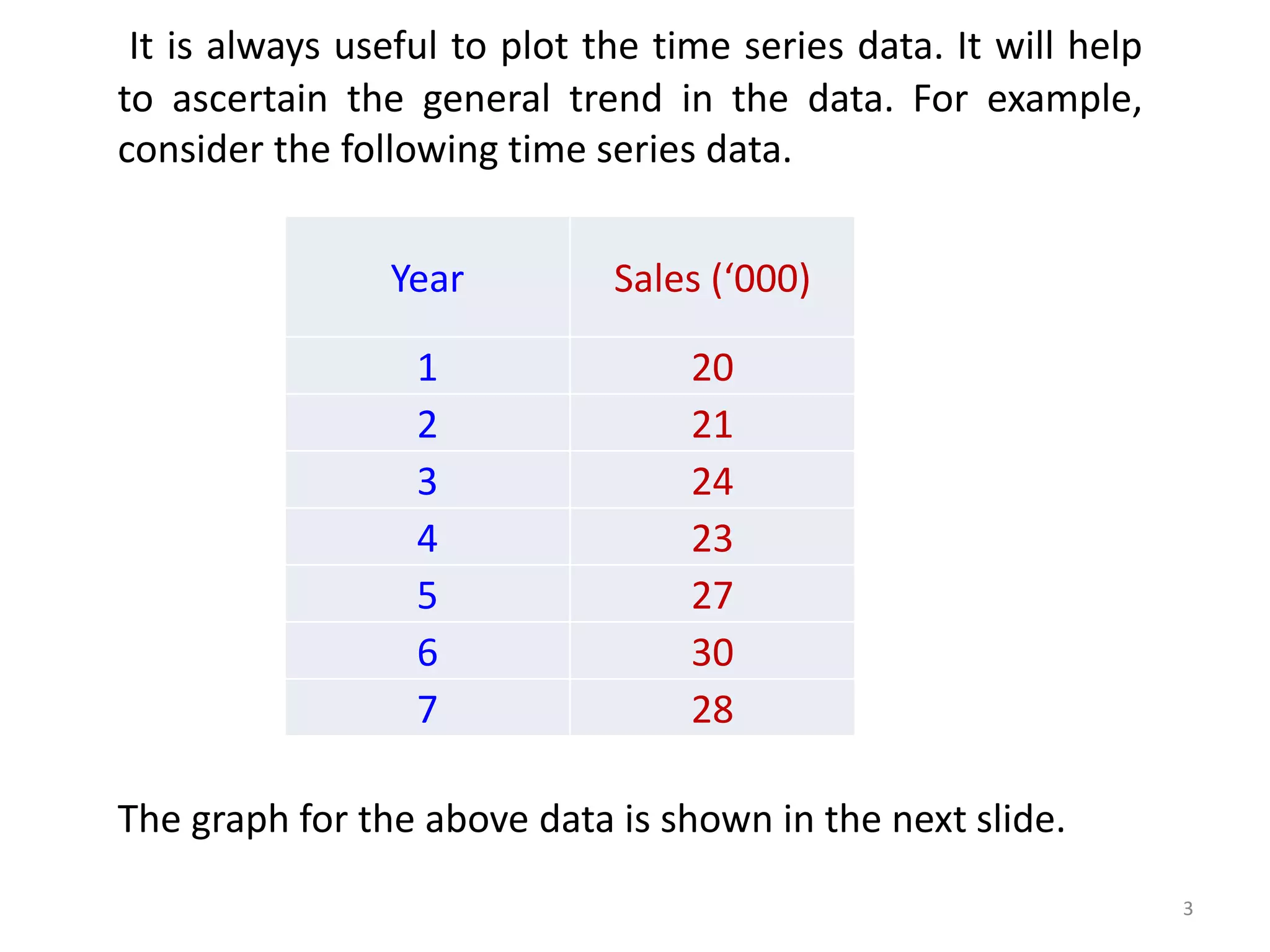
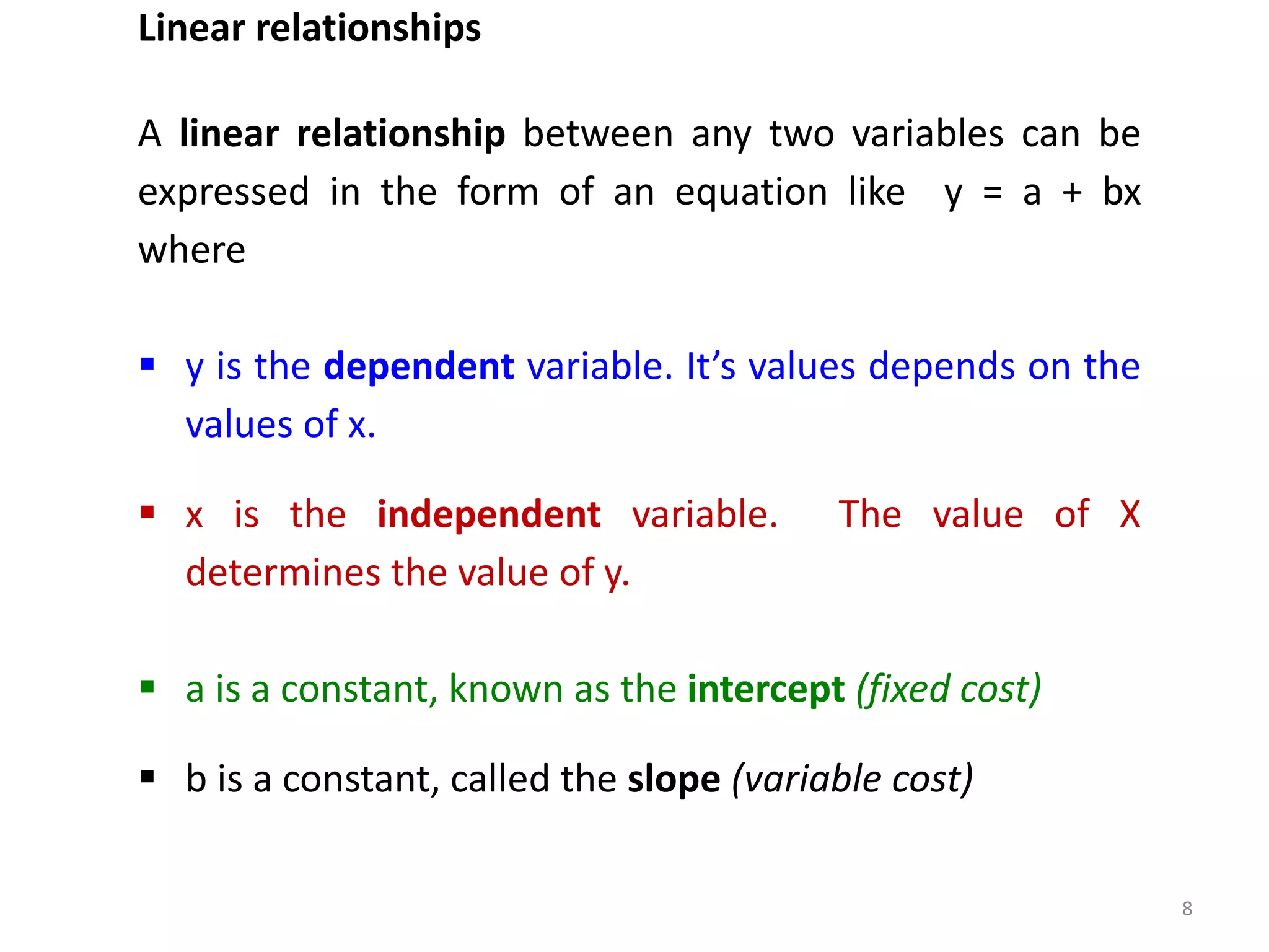
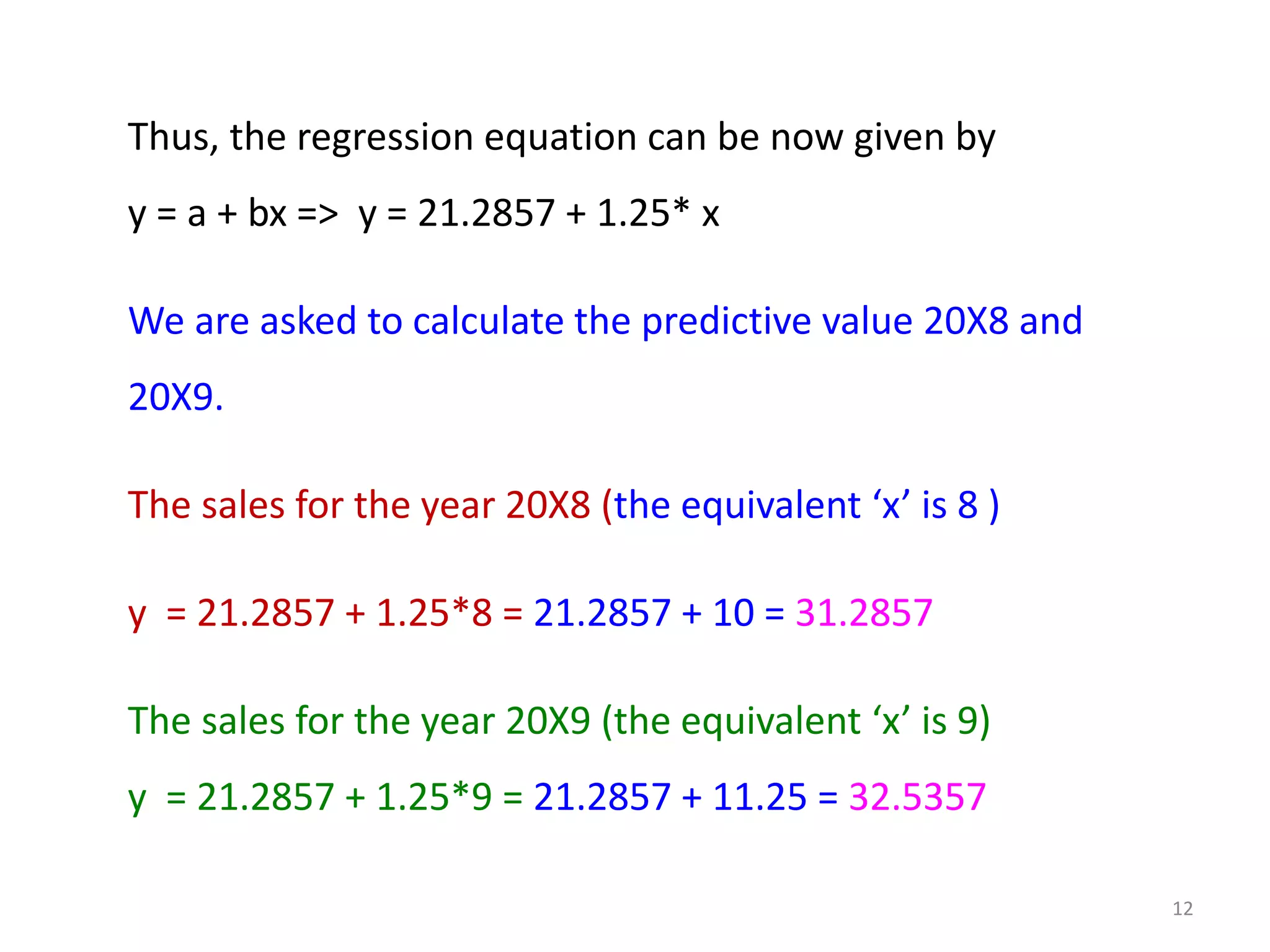
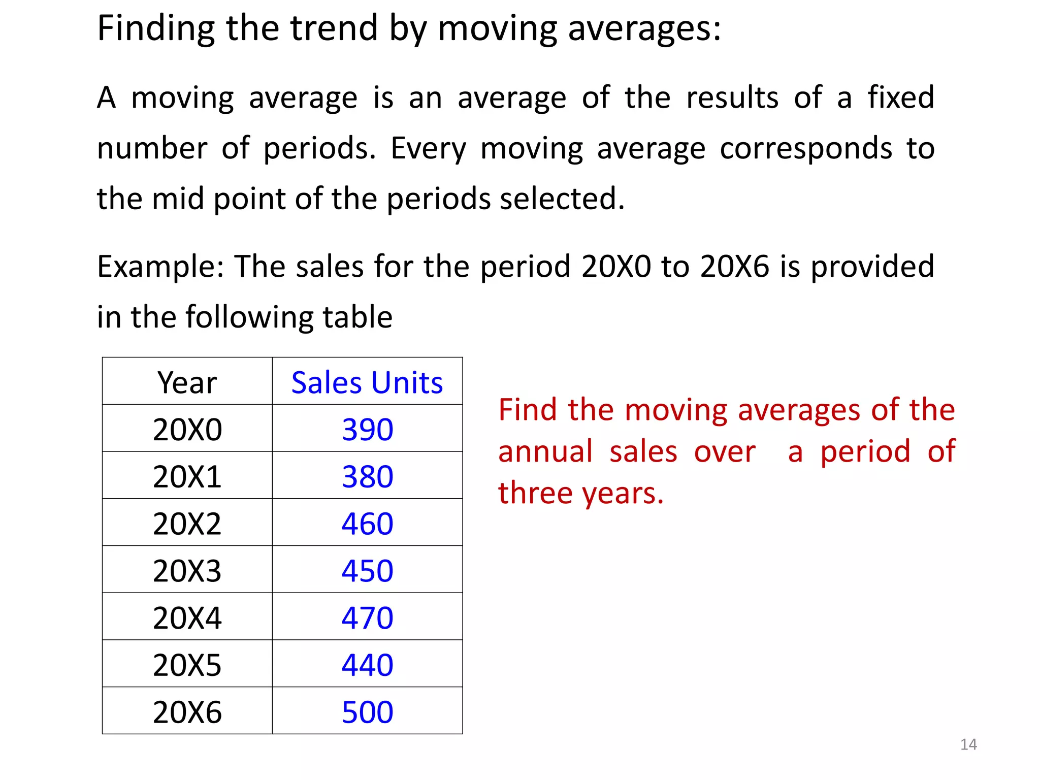
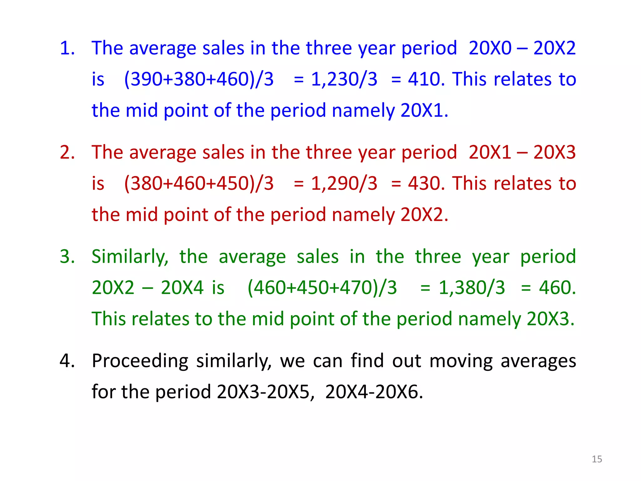
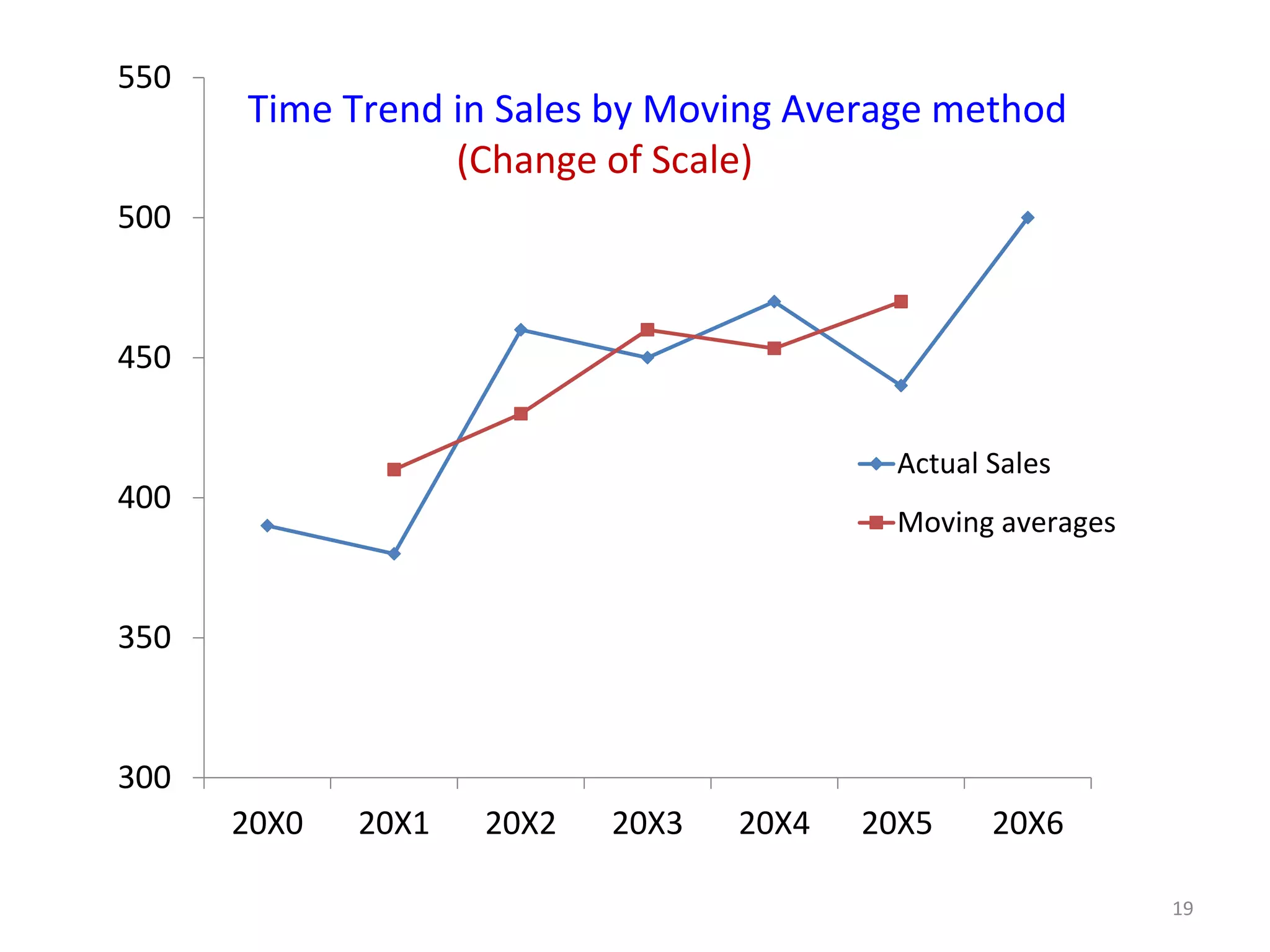
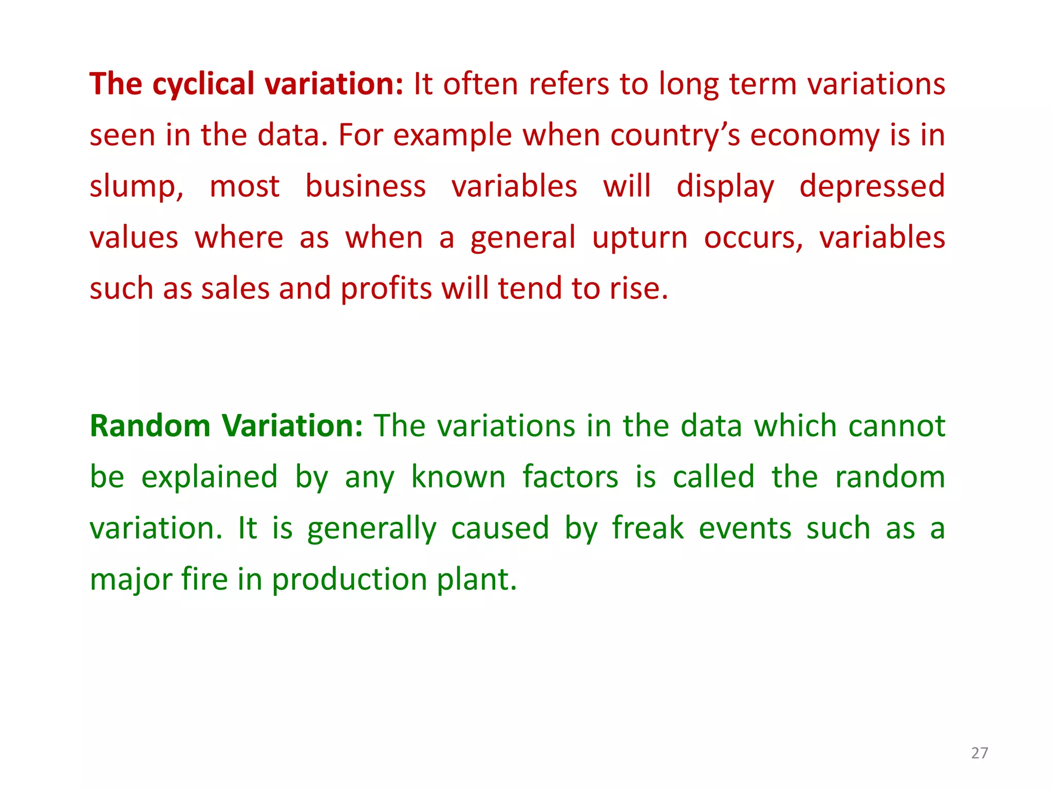
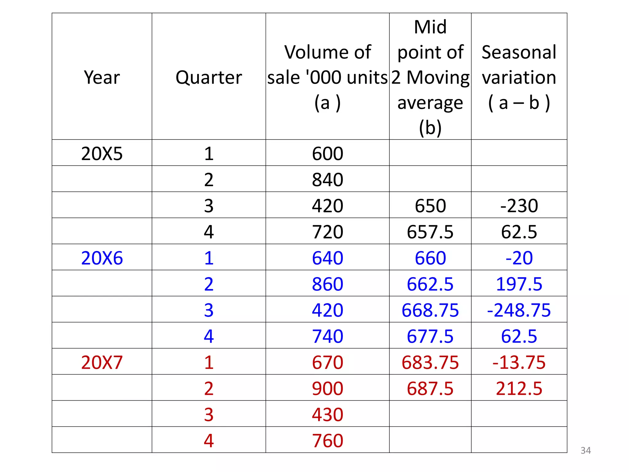
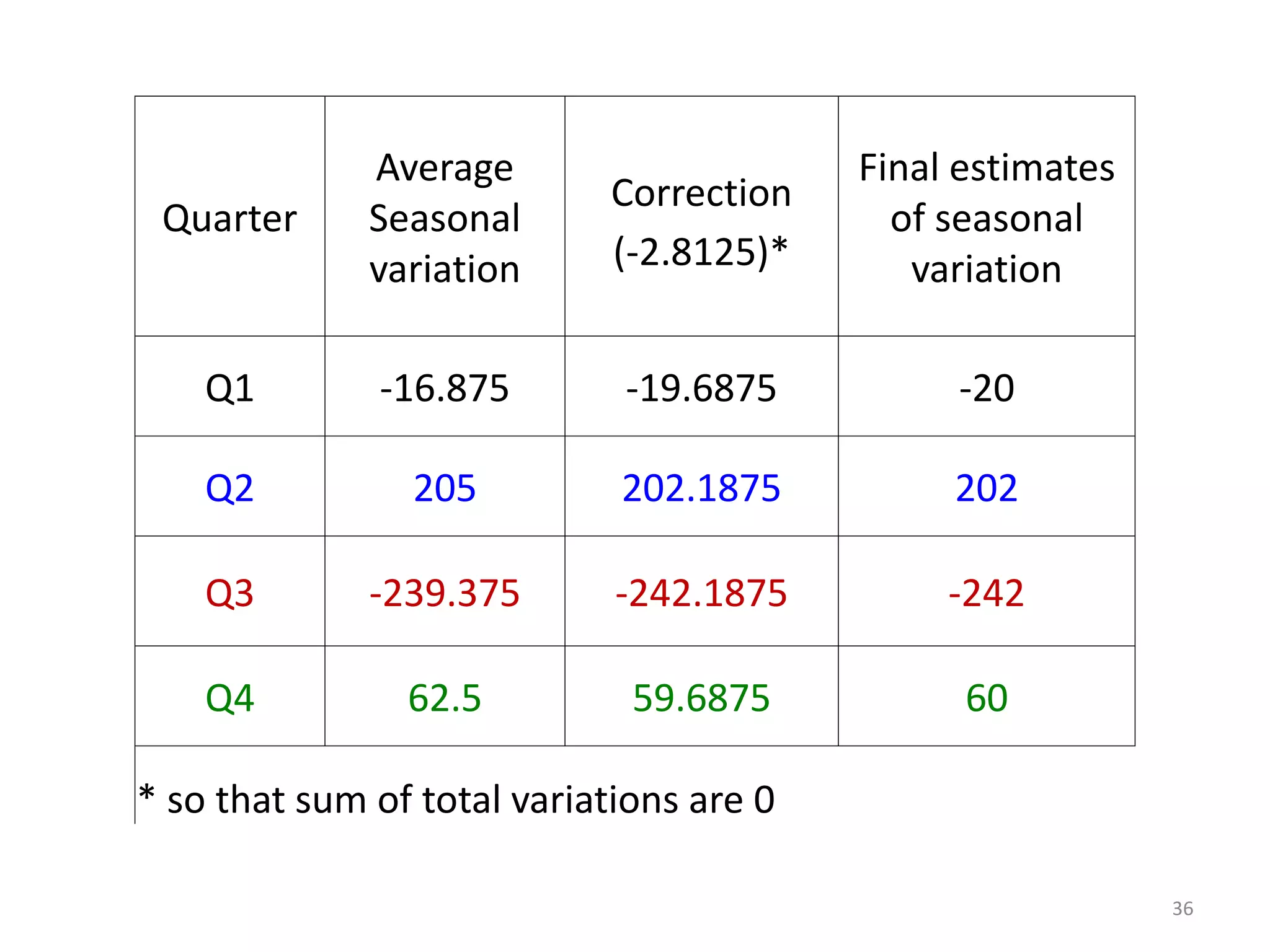
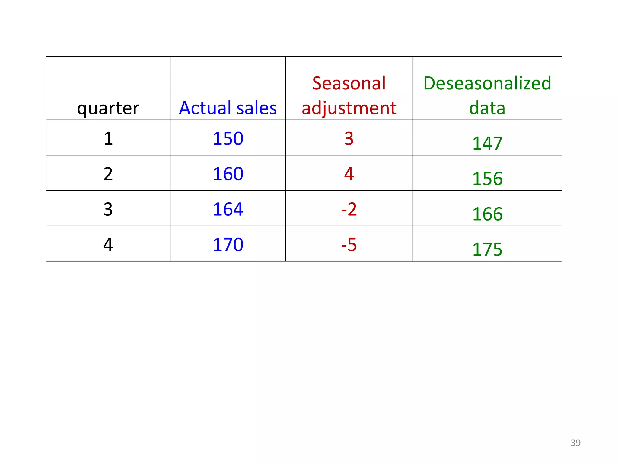
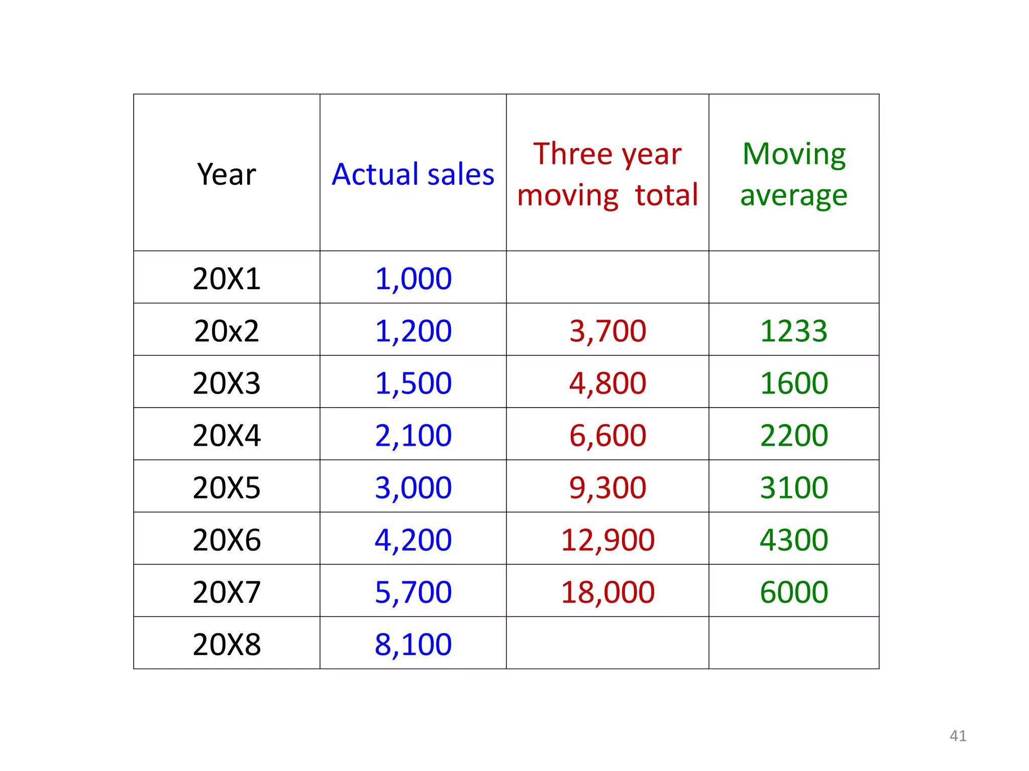
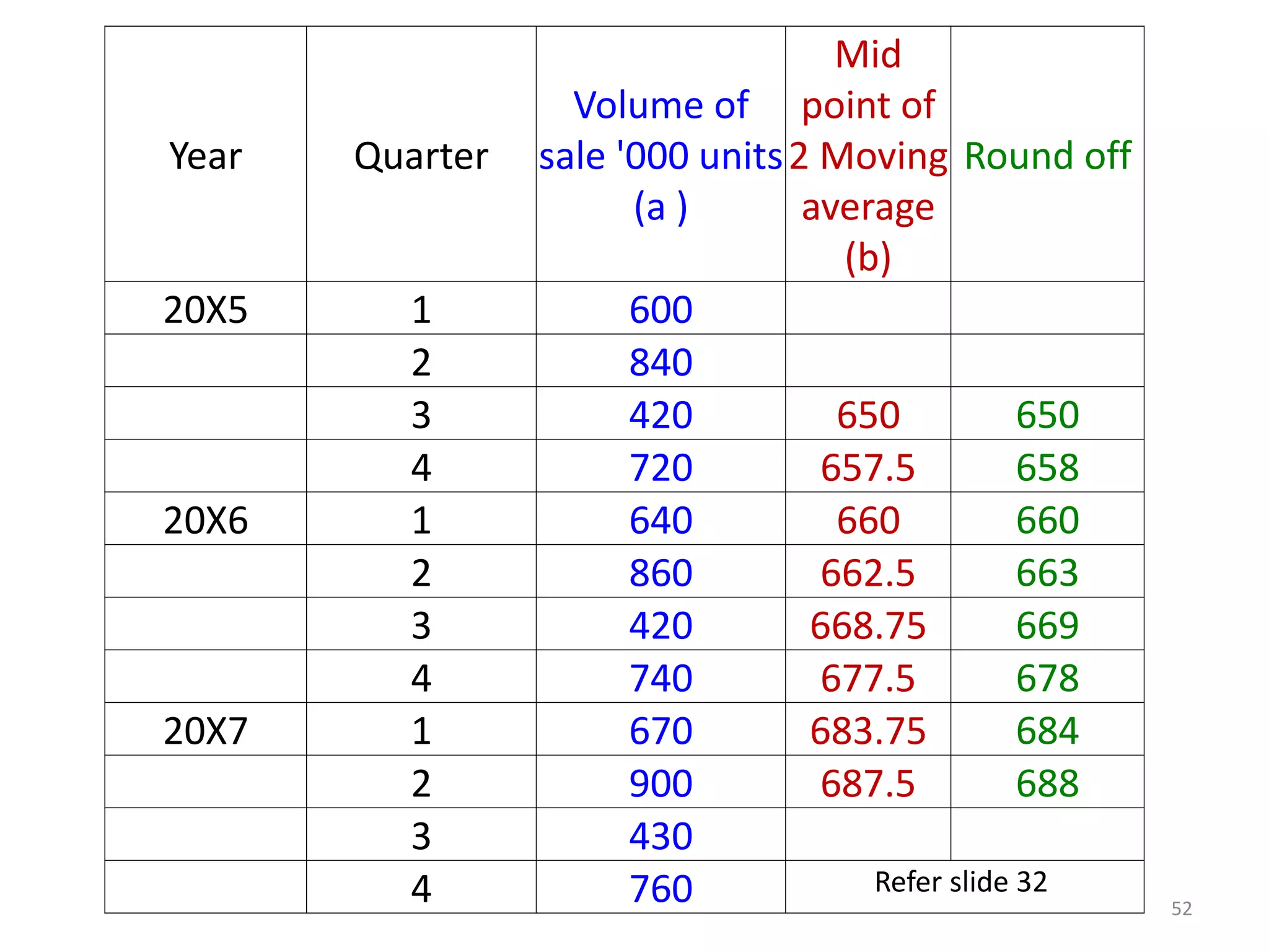
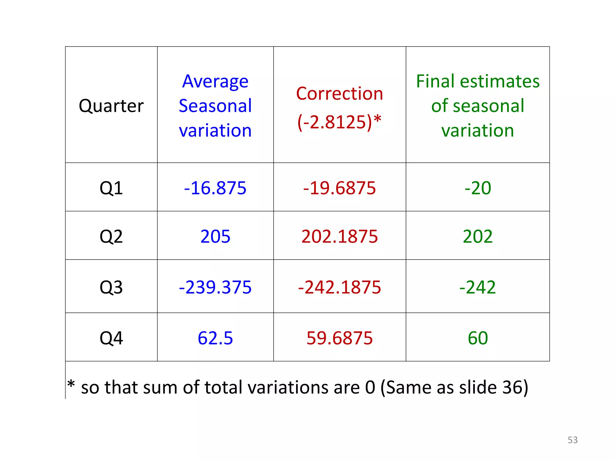
This document provides an overview of time series forecasting. It discusses key concepts such as: - Time series data that records values over time can be used for forecasting future values. Examples include factory output per day and monthly sales. - Plotting time series data helps identify trends like increasing, decreasing, or no trend over time. Regression analysis can also be used to identify linear trends and make predictions. - Moving averages smooth out fluctuations by taking the average of values over a fixed time period, like 3 years. This helps identify trends more clearly. - Components of a time series include trends, seasonal variations, cycles, and random variations. Additive and multiplicative models explain how these components combine

1. FORECASTING
(TIME SERIES)
BY
DR. RAMNATH TAKIAR
Prof. Ph.D. Programme
UNIVERSITY OF FINANCE AND ECONOMICS
ULAANBAATAR
JANUARY 2018
1

2. Time Series:
A Time series is a series of figures or values recorded over
time.
The time series data is generally useful for forecasting the
future values.
The following are the examples of time series:
 Output at a factory each day for the last month
 Monthly sales over the last two years
 Total annual costs for the last ten years
 Retail Prices Index each month for the last ten years
 The number of people employed by a company each
year for the last 20 years.
2

3. It is always useful to plot the time series data. It will help
to ascertain the general trend in the data. For example,
consider the following time series data.
Year Sales (‘000)
1 20
2 21
3 24
4 23
5 27
6 30
7 28
The graph for the above data is shown in the next slide.
3

4. 20 21
24
23
27
30
28
0
5
10
15
20
25
30
35
1 2 3 4 5 6 7
Salesin'000$
Year
Sales by different years
4
Note: A horizontal axis is always chosen to represent time, and the vertical
axis represents the values of the data recorded.

5. The trend:
It shows the general long term movement in the data over
time.
In the following examples of time series, there are three
types of trend.
Year
Output per
labour hour
Cost per unit
( $ )
Number of
Employees
4 30 1.00 100
5 24 1.08 103
6 26 1.20 96
7 22 1.15 102
8 21 1.18 103
9 17 1.25 98
Trend type A B C 5

6. 6
15
20
25
30
35
20X4 20X5 20X6 20X7 20X8 20X9
OutpurperLabourhour
Year
Trend in Output per labour hour
(20X4 - 20X9)
0.9
1
1.1
1.2
1.3
20X4 20X5 20X6 20X7 20X8 20X9
Costperunit
Year
Trend in Cost per unit (20X4 - 20X9)
88
92
96
100
104
108
20X4 20X5 20X6 20X7 20X8 20X9
NumberofEmployees
Year
Trend in Number of Employees - (20X4 - 20X9)
Decreasing trend
No trend
Increasing trend

7. 1. In time series A, there is a general downward trend in
output per labour hour (Decreasing trend).
2. In time series B, there is an upward trend in the cost
per unit (Increasing trend).
3. In time series C, there is no clear trend in the data (No
trend).
4. The presence of trend in any graph indicates that the
two variables under consideration are possibly linearly
related.
7

8. 8
Linear relationships
A linear relationship between any two variables can be
expressed in the form of an equation like y = a + bx
where
 y is the dependent variable. It’s values depends on the
values of x.
 x is the independent variable. The value of X
determines the value of y.
 a is a constant, known as the intercept (fixed cost)
 b is a constant, called the slope (variable cost)

9. 9
Linear regression analysis, also known as the 'least squares
technique', is a statistical method of finding a linear
regression line through which forecasting of dependent
variable is possible. The formulae used in the methods are:
_ _
If y = a + bx then a = ∑ y/n – b(∑x/n) = y – b x and
b = {∑xy - (∑x. ∑y)/n } / {∑x2 – (∑x)2/n} where
n is the number of pair of data for x and Y

10. 10
Regression and forecasting:
Regression method can be used to find a trend line, such as
the trend in sales over a number of periods. Let us consider
an example:
Consider the Sales of product B over the seven year period
from 20X1 to 20X7 were as follows.
Year 20X1 20X2 20X3 20X4 20X5 20X6 20X7
Sales of B 22 25 24 26 29 28 30
Calculate the trend line of sales, and forecast sales in 20X8
and 20X9 using the approach of regression analysis.

11. 11
Year x y xy x2
20X1 1 22 22 1
20X2 2 25 50 4
20X3 3 24 72 9
20X4 4 26 104 16
20X5 5 29 145 25
20X6 6 28 168 36
20X7 7 30 210 49
Total 28 184 771 140
b = {∑xy - (∑x. ∑y )/n} / {∑x2 – (∑x)2/n}
= {771 – (28 x184)/7} / {140 – (28)2/7} = 1.25
a = ∑ y/n – b(∑x/n) = 184/7 - 1.25 x (28/7) = 21.2857

12. 12
Thus, the regression equation can be now given by
y = a + bx => y = 21.2857 + 1.25* x
We are asked to calculate the predictive value 20X8 and
20X9.
The sales for the year 20X8 (the equivalent ‘x’ is 8 )
y = 21.2857 + 1.25*8 = 21.2857 + 10 = 31.2857
The sales for the year 20X9 (the equivalent ‘x’ is 9)
y = 21.2857 + 1.25*9 = 21.2857 + 11.25 = 32.5357

13. 13
Problems on Linear Regression:
Q1. The linear trend of sales of a company is $ 65,000 in
2005 and it rises by $ 2010 per year.
1) Write down the trend equation
2) If the company knows that it sales in 2015 is likely to be
10% more than the forecasted trend sales, find its expected
sales in 2015?
Q2. The trend equation fitted to a time series data is given
by Y = 1600 + 200X. The company has the production
capacity of 3600 units a year. Find after how many year will
the company's expected sales have equalled its present
production capacity?

14. Finding the trend by moving averages:
A moving average is an average of the results of a fixed
number of periods. Every moving average corresponds to
the mid point of the periods selected.
Example: The sales for the period 20X0 to 20X6 is provided
in the following table
Find the moving averages of the
annual sales over a period of
three years.
14
Year Sales Units
20X0 390
20X1 380
20X2 460
20X3 450
20X4 470
20X5 440
20X6 500

15. 1. The average sales in the three year period 20X0 – 20X2
is (390+380+460)/3 = 1,230/3 = 410. This relates to
the mid point of the period namely 20X1.
2. The average sales in the three year period 20X1 – 20X3
is (380+460+450)/3 = 1,290/3 = 430. This relates to
the mid point of the period namely 20X2.
3. Similarly, the average sales in the three year period
20X2 – 20X4 is (460+450+470)/3 = 1,380/3 = 460.
This relates to the mid point of the period namely 20X3.
4. Proceeding similarly, we can find out moving averages
for the period 20X3-20X5, 20X4-20X6.
15

16. Year Sales Units
Moving total of
successive 3
values (B )
Average value
(B/3) = trend line
20X0 390
20X1 380 1230 410
20X2 460
20X3 450
20X4 470
20X5 440
20X6 500
1st Location = (1+3)/2 =2
16

17. Year Sales Units
Moving total of
successive 3
values (B )
Average value
(B/3) = trend line
20X0 390
20X1 380 1230 410
20X2 460 1290 430
20X3 450 1380 460
20X4 470 1360 453.3
20X5 440 1410 470
20X6 500
1st Location = (1+3)/2 =2; 2ND Location = (2+4)/2 =3; 3rd Location = (3+5)/2=4 ;
4th Location = (4+ 6)/2 = 5; 5th Location = (5+7)/2=6 17

18. 0
100
200
300
400
500
600
20X0 20X1 20X2 20X3 20X4 20X5 20X6
Actual Sales
Moving averages
Time Trend in Sales by Moving Average method
(Original Scale )
18

19. 300
350
400
450
500
550
20X0 20X1 20X2 20X3 20X4 20X5 20X6
Actual Sales
Moving averages
Time Trend in Sales by Moving Average method
(Change of Scale)
19

20. Note the following:
1. The moving average series has five figures relating to
the years 20X1 to 20X5. The original series had seven
figures for the years 20X0 to 20X6.
2. The moving average series is having two observations
less than the original series. In general for 3 years
moving average, if the original series have (n)
observations the trend values will always have ( n-2 )
observations.
3. There is an upward trend in sales, which is more
noticeable from the series of moving averages than
from the original series of actual sales every year.
20

21. Example of moving averages for even number of
periods:
Year Sales Units
20X0 390
20X1 380
20X2 460
20X3 450
20X4 470
20X5 440
20X6 500
20X7 520
Take a moving average of the annual sales over a period
of four years.
21

22. Year Location
Sales
Units
Moving
total of 4
values
(B )
Average
value
(B/4)
Mid point
of 2
moving
averages –
trend line
20X0 1 390
20X1 2 380
20X2 3 460 1680 420.0
20X3 4 450
20X4 5 470
20X5 6 440
20X6 7 500
20X7 8 520
1st Loaction = (1+4)/2 =2.5
22

23. Year Location
Sales
Units
Moving
total of 4
values
(B )
Average
value
(B/4)
Mid point
of 2
moving
averages –
trend line
20X0 1 390
20X1 2 380
20X2 3 460 1680 420.0
20X3 4 450 1760 440.0
20X4 5 470
20X5 6 440
20X6 7 500
20X7 8 520
1st Loaction = (1+4)/2 =2.5; 2nd Location = (2+5)/4 = 3.5
23

24. Year Location
Sales
Units
Moving
total of 4
values
(B )
Average
value
(B/4)
Mid point
of 2
moving
averages –
trend line
20X0 1 390
20X1 2 380
20X2 3 460 1680 420.0 430.0
20X3 4 450 1760 440.0 447.5
20X4 5 470 1820 455.0 460.0
20X5 6 440 1860 465.0 473.8
20X6 7 500 1930 482.5
20X7 8 520
1st Loaction = (1+4)/2 =2.5; 2nd Location = (2+5)/4 = 3.5; 3rd Location = (3+6)/2 = 4.5;
4th Location = (4+7)/2 = 5.5; 5th Location = (5+8)/2 = 6.5 24

25. 350
370
390
410
430
450
470
490
510
530
20X0 20X1 20X2 20X3 20X4 20X5 20X6 20X7
Actual sales values
Moving average values
Time Trend in Sales by Moving Average method
(4 years Moving Average)
25

26. There are four components of a time series:
 Trend
 Seasonal variations
 Cycle or cyclic variations and
 random variations or residual variation.
Trend: The trend in a time series is the general, overall
movement of the data with any sharp fluctuations largely
smoothed out. It is often called the underlying trend.
Seasonal Variation: A variation in data which you can
observe with respect to season is called the seasonal
variation. In general, if the data is recorded weekly,
monthly or quarterly, it will tend to display the seasonal
variations. In case of annual recording, it is not possible.
26

27. The cyclical variation: It often refers to long term variations
seen in the data. For example when country’s economy is in
slump, most business variables will display depressed
values where as when a general upturn occurs, variables
such as sales and profits will tend to rise.
Random Variation: The variations in the data which cannot
be explained by any known factors is called the random
variation. It is generally caused by freak events such as a
major fire in production plant.
27

28. There are two models by which the Time Series data can be
analyzed:
1) Additive model;
2) Multiplicative model
In Additive model the four components are assumed to add
together to give the variable Y.
Y = T + S + C + R
In multiplicative model the above components are
multiplied to give Y.
Y = T x S x C x R
We will discuss both the models with example, little later.
28

29. Seasonal variations:
Seasonal variations are short term fluctuations in recorded
values due to different times of the year, on different days
of the week or at different times of the day.
Examples of seasonal variations:
1. Sales of ice cream will be higher in summer than winter.
2. The telephone network may be heavily used at certain
times of the day (such as mid-morning and mid-
afternoon.
3. Sales of winter coats will be higher in winter than in
summer.
4. Travelling will be higher when schools/colleges are
closed.
29

30. Finding the Seasonal variations:
 First, find the trend values by moving average method
 Seasonal variation is the difference between the actual
and the trend values (additive model).
 In case of more than one values obtained for same
season, its average can be taken to represent the
seasonal variation.
30

31. Year Quarter
Volume of sale
'000 units
20X5 1 600
2 840
3 420
4 720
20X6 1 640
2 860
3 420
4 740
20X7 1 670
2 900
3 430
4 760
Find out the seasonal variation for sales data of Linden Ltd.
31

32. Year Quarter
Volume of
sale '000
units
Moving
total of 4
values
Average
Mid point
of 2
Moving
averages
20X5 1 600
2 840
3 420 2580 645 650*
4 720 2620 655 657.5**
20X6 1 640 2640 660 660
2 860 2640 660 662.5
3 420 2660 665 668.75
4 740 2690 672.5 677.5
20X7 1 670 2730 682.5 683.75
2 900 2740 685 687.5
3 430 2760 690
4 760
* - (645+655)/2 = 650; ** - (655+660)/2=657.5 32

33. 0
200
400
600
800
1000
1 2 3 4 1 2 3 4 1 2 3 4
20X5 20X6 20X7
Sales Volume of sales quarters - Linden Ltd.
Actual sales
Trend sales
33

34. Year Quarter
Volume of
sale '000 units
(a )
Mid
point of
2 Moving
average
(b)
Seasonal
variation
( a – b )
20X5 1 600
2 840
3 420 650 -230
4 720 657.5 62.5
20X6 1 640 660 -20
2 860 662.5 197.5
3 420 668.75 -248.75
4 740 677.5 62.5
20X7 1 670 683.75 -13.75
2 900 687.5 212.5
3 430
4 760 34

35. Quarter 20X5 20X6 20X7 Total
Average
Seasonal
variation
Q1 -20 -13.75 -33.75 -16.875
Q2 197.5 212.5 410 205
Q3 -230 -248.75 -478.75 -239.375
Q4 62.5 62.5 125 62.5
total 11.25
Average Error = 11.25/4 = 2.8125
35
The average error can be taken as the random variation present in the trend values

36. Quarter
Average
Seasonal
variation
Correction
(-2.8125)*
Final estimates
of seasonal
variation
Q1 -16.875 -19.6875 -20
Q2 205 202.1875 202
Q3 -239.375 -242.1875 -242
Q4 62.5 59.6875 60
* so that sum of total variations are 0
36

37. Year Quarter
Volume of
sale '000
units
Adjustment
for season
Adjusted
sales for
season
20X5 1 600 -20 620
2 840 202 638
3 420 -242 662
4 720 60 660
20X6 1 640 -20 660
2 860 202 658
3 420 -242 662
4 740 60 680
20X7 1 670 -20 690
2 900 202 698
3 430 -242 672
4 760 60 700
Adjustment for seasonal variation in sales
37

38. quarter Actual sales
Seasonal
adjustment
Deseasonalized
data
1 150 3 147
2 160 4 156
3 164 -2 166
4 170 -5 175
39

39. A weakness in moving average analysis:
The moving average calculations so far shown are based on
additive model which means we add the values for a
number of periods and take the average of those values.
An additive model has the important drawback that when
there is a consistent rising or declining trend, the moving
average trend will show either higher or lower values as
compared to actual values.
Consider the following example:
40

40. Year Actual sales
Three year
moving total
Moving
average
20X1 1,000
20x2 1,200 3,700 1233
20X3 1,500 4,800 1600
20X4 2,100 6,600 2200
20X5 3,000 9,300 3100
20X6 4,200 12,900 4300
20X7 5,700 18,000 6000
20X8 8,100
41

41. Note the following:
1. The trend values are always higher compared to actual
values.
2. Thus, The trend sales is not a good representation of
actual sales.
3. The trend values cannot be used for forecasting.
42

42. Seasonal variation using the multiplicative
model:
In additive model, the seasonal variation was assumed
to be fixed, while in the multiplicative model the
seasonal variation is assumed to be proportional to
trend values
The proportional (multiplicative) model summarizes a
time series as Y = T X S X R or (Y = T*S*R) where T is for
trend, S is for seasonal variation and R is for Random
variation.
43

43. Year Quarter
Volume of
sale '000
units (Y )
Trend
values ( T )
(Refer slide 32)
Seasonal %
( Y/T)
20X5 1 600
2 840
3 420 650 0.646
4 720 657.5 1.095
20X6 1 640 660 0.970
2 860 662.5 1.298
3 420 668.75 0.628
4 740 677.5 1.092
20X7 1 670 683.75 0.980
2 900 687.5 1.309
3 430
4 760
44

44. Quarter 20X5 20X6 20X7 Total
Average
Seasonal
variation
Q1 0.970 0.980 1.950 0.975
Q2 1.298 1.309 2.607 1.304
Q3 0.646 0.628 1.274 0.637
Q4 1.095 1.092 2.187 1.094
Correction = 0.009/4 = 0.00225 total 4.009
45

45. Quarter
Average
Seasonal
variation
Final estimates
= actual -
Correction
(0.0025)*
Q1 0.975 0.972
Q2 1.304 1.301
Q3 0.637 0.635
Q4 1.094 1.091
46

46. Year Quarter
Volume of
sale '000
units ( Y )
Adjustment
for season
( T)
Adjusted
sales for
season ( Y/T)
20X5 1 600 0.972 617*
2 840 1.301 646
3 420 0.635 662
4 720 1.091 660
20X6 1 640 0.972 658
2 860 1.301 661
3 420 0.635 662
4 740 1.091 678
20X7 1 670 0.972 689
2 900 1.301 692
3 430 0.635 678
4 760 1.091 697
47* 600/0.972 = 617

47. Comparison of season adjusted sales by additive and
multiplicative model
Year Quarter
Volume of
sale '000
units
Season adjusted values
Additive
model
Multiplicative
model
20X5 1 600 620 617
2 840 638 646
3 420 662 662
4 720 660 660
20X6 1 640 660 658
2 860 658 661
3 420 662 662
4 740 680 678
20X7 1 670 690 689
2 900 698 692
3 430 672 678
4 760 700 697 48

48. Note:
 The multiplicative model is better than the additive
model when the trend is increasing or decreasing over
time. In such circumstances, seasonal variations are
likely to be increasing or decreasing too.
 In additive models, the season effect is assumed to be
fixed which is not proper when there is a clear cut
increasing or decreasing trend.
 In the multiplicative model the increasing or decreasing
trend values are multiplied by a seasonal variation
factor, thus taking into account of the changing seasonal
variations.
49

49. Sales forecasting : time series analysis
The main idea behind time series analysis is the
identification of the trend in the data and its separation
from seasonal variation. Once that has been done forecasts
of future values can be made as follows:
1. The trend line should be calculated.
2. The trend line should be used to forecast future trend
line values.
3. These values should be adjusted by the average
seasonal variation applicable to the future period, to
determine the forecast for the period.
Extending the trend line outside the range of known data
to forecast the values for future is known as extrapolation. 50

50. There are two other principle methods of calculating the
forecast trend line.
Inspection:
The trend line can be drawn by eye on a graph in such a
way that it appears to lie evenly between the recorded
points. Forecasts can then be read off of an extrapolated
trend line.
Common sense “rule of thumb approach”
This method is simply to guess what future movements in
the trend line might be, based on the movements in the
past. It is not a mathematical technique, merely a common
sense, rule of thumb approach.
51

51. Year Quarter
Volume of
sale '000 units
(a )
Mid
point of
2 Moving
average
(b)
Round off
20X5 1 600
2 840
3 420 650 650
4 720 657.5 658
20X6 1 640 660 660
2 860 662.5 663
3 420 668.75 669
4 740 677.5 678
20X7 1 670 683.75 684
2 900 687.5 688
3 430
4 760 Refer slide 32
52

52. Quarter
Average
Seasonal
variation
Correction
(-2.8125)*
Final estimates
of seasonal
variation
Q1 -16.875 -19.6875 -20
Q2 205 202.1875 202
Q3 -239.375 -242.1875 -242
Q4 62.5 59.6875 60
* so that sum of total variations are 0 (Same as slide 36)
53

53. Note the following:
The estimated trend values for
20X5 – 3rd quarter is 650
20x7 – 2nd quarter is 688
Calculate the increase over 7 quarters is 688-650 = 38
Therefore the average increase per quarter is 38/7 = 5.43  5
Forecast for
20X7 – 3rd quarter = 688 + 5 = 693
20X7 – 4th quarter = 688 + (2*5) = 688 + 10 = 698
54

54. Adjusting for seasonal trend we get :
20X7 – 3rd quarter = 693 - 242 = 451
20X7 – 4th quarter = 698 + 60 = 758
So, the projected sales for 3rd and 4th quarter of 20X7 is
451,000 and 758,000 units.
55

55. Quarter
Average
Seasonal
variation
Final estimates
= actual -
Correction
(0.0025)*
Q1 0.975 0.972
Q2 1.304 1.301
Q3 0.637 0.635
Q4 1.094 1.091
56
Same as slide 42

56. Adjusting for seasonal trend by MULTIPLICATIVE approach we
get :
20X7 – 3rd quarter = 693*0.635 = 440.055 ≈ 440
20X7 – 4th quarter = 698*1.094= 763.612 ≈ 764
So, the projected sales for 3rd and 4th quarter of 20X7 is
440,055 and 763,600 units.
57

57. Year Quarter
Volume
of sale
'000 units
Trend
value
Average
seasonal
variation
1 1 18
2 30
3 20 18.75
4 6 19.375
2 1 20 20 -0.1
2 33 20.5 12.4
3 22 21 1.1
4 8 21.5 -13.4
3 1 22 22.125
2 35 22.75
3 25
4 10
Sales of product X each quarter for the last three years ,
including trend and seasonal variation are as follows:
Forecast sales of year 4 for each quarter ?
58

58. Use the trend line and estimate the seasonal variations to
forecast sales in each quarter of year 4. Class work
Forecast problems:
1. Forecasting beyond range for many years will not be
reliable.
2. If less data is available for forecast, the reliability of
the forecast will also be less.
3. The pattern of trend and seasonal variations can not
be guaranteed to continue in the future.
4. There is always a danger of random variations
upsetting the pattern of trend and seasonal variation
and thereby reducing the reliability of the forecasting
values. 59

59. 60