Seminar 10 BIOSTATISTICS

Seminar 10 BIOSTATISTICS

• 1.
  TESTS OF SIGNIFICANCE Dr.ANUSHA DIVVI 2ND YEAR POST GRADUATE DEPARTMENT OF PUBLIC HEALTH DENTISTRY
• 2.
  CONTENTS • Introduction • Dataand Types • Measures of central tendency • Measures of dispersion • Hypothesis and types • Errors
• 3.
  • Power, Levelof significance, effect size • Parametric tests • Non Parametric tests • Flowchart for deciding appropriate statistical test • Conclusion • References
• 4.
  INTRODUCTION Statistics is amathematical science which deals with the methods of collecting, compiling, presenting, interpreting the numerical data and making inferences/drawing conclusions based on the analysis of data Gordon B. Drummond Statistics: all together now, one step at a time; Adv Physiol Educ 2011:35;129
• 5.
  • Biostatistics –Branch of statistics • John Graunt (1620 – 1674) is the father of biostatistics • Biostatistics can be divided into two subcategories: • Descriptive biostatistics • Inferential biostatistics
• 6.
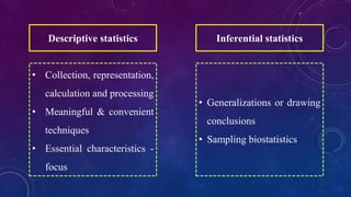
  Descriptive statistics • Collection,representation, calculation and processing • Meaningful & convenient techniques • Essential characteristics - focus Inferential statistics • Generalizations or drawing conclusions • Sampling biostatistics
• 7.
  DATA • Data isa collection of facts, such as numbers, words, measurements, observations or even just descriptions of things. • The singular form is "datum"
• 8.
  TYPES OF DATA 1.Qualitative / Categorical data • Nominal • Ordinal 2. Quantitative / Measurement data • Discrete • Continuous
• 9.
  CATEGORICAL DATA • Variablebeing measured is grouped into categories • Resulting data are merely labels or categories Classified as: • Nominal(Nominal / Binary or Dichotomous) • Ordinal
• 10.
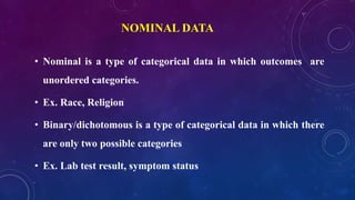
  NOMINAL DATA • Nominalis a type of categorical data in which outcomes are unordered categories. • Ex. Race, Religion • Binary/dichotomous is a type of categorical data in which there are only two possible categories • Ex. Lab test result, symptom status
• 11.
  ORDINAL DATA • Atype of categorical data in which natural order is important • Interval between categories is not meaningful • Ex. Pain: Mild, moderate, severe
• 12.
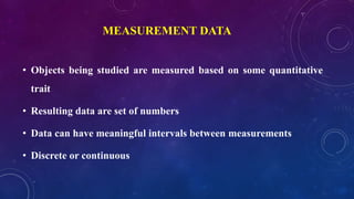
  MEASUREMENT DATA • Objectsbeing studied are measured based on some quantitative trait • Resulting data are set of numbers • Data can have meaningful intervals between measurements • Discrete or continuous
• 13.
  DISCRETE DATA • Discretedata – only certain values are possible • There are gaps between the possible values • Ex. No. of missing teeth, No of lesions in mouth
• 14.
  CONTINUOUS DATA • Continuousmeasurement data means any value within an interval is possible • Ex. Mouth opening, Distances between teeth
• 15.
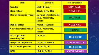
  Data Denoted byType of variables Gender Male, Female Hair colour Black, Grey, Red Dental fluorosis grades Normal, Questionable, Mild, Moderate, Severe Dental caries Present / Absent Chronic Periodontitis Mild, Moderate, Severe No. of patients attending OP 10,15,25 Height of the patient 170.5 cm, 180 cm No. of teeth present 23, 24, 28, 32 BMI 19.4, 21.5, 25.5 ORDINAL NOMINAL NOMINAL NOMINAL ORDINAL DISCRETE DISCRETE CONTINUOUS CONTINUOUS 15
• 16.
  MEASURES OF CENTRALTENDENCY • Tendency of the observations towards the central point of data • A single number • Measures of central location • Summary Statistics • Representative of the entire data • Mean, median, mode
• 17.
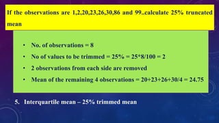
  • Mean –Average of the values of all the variables Types 1. Arithmetic mean 2. Geometric mean – when values change exponentially 3. Harmonic mean – reciprocal of arithmetic mean 4. Truncated mean – trimmed mean 5. Interquartile mean – 25% trimmed mean If the observations are 1,2,20,23,26,30,86 and 99..calculate 25% truncated mean • No. of observations = 8 • No of values to be trimmed = 25% = 25*8/100 = 2 • 2 observations from each side are removed • Mean of the remaining 4 observations = 20+23+26+30/4 = 24.75
• 18.
  • Median: Themiddle value when all the variables are arranged in an order ( either ascending or descending) • Mode : The most repeated value • Mode = 3 median – 2 mean
• 19.
  • The meanhas one main disadvantage: it is particularly susceptible to the influence of outliers. • These are values that are unusual compared to the rest of the data set by being especially small or large in numerical value.
• 20.
  • For example,consider the wages of staff at a factory below: Staff 1 2 3 4 5 6 7 8 9 10 Salary 15k 18k 16k 14k 15k 15k 12k 17k 90k 95k • Mean salary for these ten staff is 30.7k • Mean is being skewed by the two large salaries • Therefore, in this situation consider median
• 21.
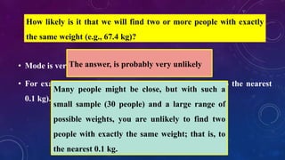
  • Mode isvery rarely used with continuous data • For example, consider measuring 30 peoples' weight (to the nearest 0.1 kg). How likely is it that we will find two or more people with exactly the same weight (e.g., 67.4 kg)? The answer, is probably very unlikely Many people might be close, but with such a small sample (30 people) and a large range of possible weights, you are unlikely to find two people with exactly the same weight; that is, to the nearest 0.1 kg.
• 22.
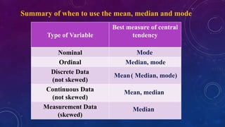
  Summary of whento use the mean, median and mode Type of Variable Best measure of central tendency Nominal Ordinal Discrete Data (not skewed) Continuous Data (not skewed) Measurement Data (skewed) Mean( Median, mode) Mean, median Median Mode Median, mode
• 23.
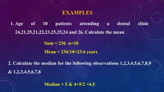
  EXAMPLES 1. Age of10 patients attending a dental clinic 24,21,25,21,22,23,25,25,24 and 26. Calculate the mean Sum = 236 n=10 Mean = 236/10=23.6 years Median = 5 & 4+5/2 =4.5 2. Calculate the median for the following observations 1,2,3,4,5,6,7,8,9 & 1,2,3,4,5,6,7,8
• 24.
  3. What isthe mode for the following observations A+, O+, B+, A+, A+, A-, A+,A+ Mode = A+
• 25.
  MEASURES OF DISPERSION •Degree of spread or variation of the variable about a central value Range: It is the difference between the highest and lowest observations. Ex. Diastolic BP of 5 individuals is 90,80,78,84,98. Highest observation is 98 Lowest observation is 78 Range is 98-78= 20.
• 26.
  Mean deviation • Averageof the deviations from the arithmetic mean • M.D. = ∑ X-Xi /n • X – arithmetic mean • Xi – value of each observation in the data • N= number of observations • Calculate the mean deviation of the data 3, 6, 6, 7, 8, 11, 15, 16
• 27.
  • Mean =72/8 = 9 • Value Distance from 9 3 6 6 3 6 3 7 2 8 1 11 2 15 6 16 7 • Mean deviation = 30/8 = 3.75
• 28.
  Quartile deviation • Itis based on the lower quartile Q1 and upper quartile Q3. • Q1 = 25*n/100 Q3 = 75*n/100 • The difference Q3 - Q1 is called the inter quartile range. • The difference Q3 - Q1 divided by 2 is called semi-inter-quartile range or the quartile deviation. • Q.D = Q3 - Q1 /2 Suppose the values of X are 20, 12, 18, 25, 32, 10, 35 Calculate inter quartile range and quartile deviation of the data
• 29.
  • Arrange thegiven data in ascending or descending order • X = 10, 12, 18, 20, 25, 32,35 • No. of items = 7 • Q1 = 25*7/100 = 1.75 (rounded to 2nd) = 12 • Q3 = 75*6/100 = 5.25th item (rounded to 5th) = 25 • Inter-quartile range = Q3 – Q1 = 25-12= 13 • Quartile deviation = 13/2 = 6.5
• 30.
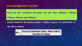
  STANDARD DEVIATION • Squareroot of the mean of the squared deviations from the arithmetic mean • Small standard deviation means a higher degree of uniformity of the observations valuesofNumber Value)Mean-Valuel(IndividuaofSum SD 2  Find out the standard deviation for the data 600mm, 470mm, 170mm, 430mm and 300mm.
• 31.
  • Mean =1970/5 = 394 • Calculate variance - take each difference, square it, and then average the result: • Standard Deviation • σ= √21,704 = 147.32... = 147 (to the nearest mm)
• 32.
  HYPOTHESIS • A hypothesiscan be defined as a tentative prediction or explanation of the relationship between two or more variables. • A supposition arrived at from observation or reflection • A hypothesis helps to translate the research problem & objectives into a clear explanation or prediction of the expected results or outcomes of the research study
• 33.
  A clearly statedhypothesis includes: • Variables to be manipulated or measured • Identifies the population to be examined • Indicates the proposed outcome for the study
• 34.
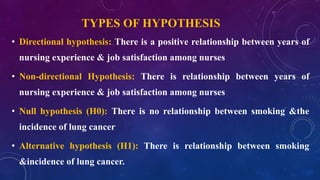
  TYPES OF HYPOTHESIS •Directional hypothesis: There is a positive relationship between years of nursing experience & job satisfaction among nurses • Non-directional Hypothesis: There is relationship between years of nursing experience & job satisfaction among nurses • Null hypothesis (H0): There is no relationship between smoking &the incidence of lung cancer • Alternative hypothesis (H1): There is relationship between smoking &incidence of lung cancer.
• 35.
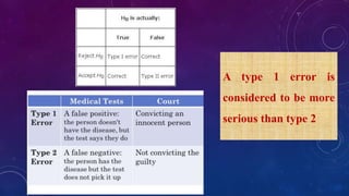
  ERRORS • Mistakes regardingthe relationship between the two variables • In 1928, Jerzy Neyman and Egon Pears – 2 errors • Type I error: Rejection of true null hypothesis • Accept the null hypothesis and reject the alternate hypothesis, but the opposite occurs. • Probability - alpha
• 36.
  • Type IIerror : Accepting false null hypothesis • Reject the null hypothesis and accept the alternate hypothesis, but the opposite occurs • Probability - beta
• 37.
  A type 1error is considered to be more serious than type 2
• 38.
  In this example,which type of error would you prefer to commit? • Null Hypothesis: The new mouthwash is no better at treating chronic periodontitis than the old mouthwash • Research Hypothesis: The new mouthwash is better at treating chronic periodontitis than the old mouthwash
• 39.
  • If aType I error is committed, the null hypothesis should be accepted, but it is rejected • People may be treated with the new mouthwash, when they would have been better off with the old one • If a Type II error is committed, the null hypothesis should be rejected, but it is accepted • People may not be treated with the new mouthwash, although they would be better off than with the old one
• 40.
  LEVEL OF SIGNIFICANCE •Researchers generally specify the probability of committing a Type I error that they are willing to accept, i.e., the value of alpha. • Most researchers select an alpha=0.05 • This means that they are willing to accept a probability of 5% of making a Type I error
• 41.
  POWER • The probabilitythat the researcher will make a correct decision to reject the null hypothesis when it is really false • More power = less risk for a type 2 error • Usually set at 0.8 or greater before a study begins
• 42.
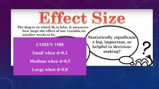
  COHEN 1988 Small whend=0.2 Medium when d=0.5 Large when d=0.8
• 43.
  ‘p’ value • Probabilityof occurrence of the differences in values due to chance or otherwise • Evidence against null hypothesis • Smaller p value – more evidence • <0.05
• 44.
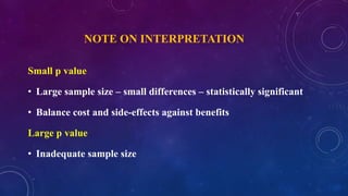
  NOTE ON INTERPRETATION Smallp value • Large sample size – small differences – statistically significant • Balance cost and side-effects against benefits Large p value • Inadequate sample size
• 45.
  • P valueindicates only the role of chance but not the precision of the observed effect size • To overcome this a more informative measure - Confidence interval is reported
• 46.
  Confidence level • Confidencelevel = 1-alpha • So if your level of significance is 0.05, the corresponding confidence level is 95% • Probability of any difference falling outside 95% is only 0.05 • 95% confident that true mean of population will fall within the given range of values • Confidence level may also be fixed at 90%, 99%, 99.9%
• 47.
  CONFIDENCE LIMITS • Loweand upper boundaries which define the range of confidence interval • The limits of 95% confidence interval will be x +/- 1.96 SE • For example if the sample mean is 180 mg/dl and the standard error is 15mg, then the confidence limits are 150.6 and 209.4 mgs/dl
• 48.
  CONFIDENCE INTERVAL • Rangebetween lower and upper boundaries of confidence limits • An interval calculated at a 95% level means we are 95% confident that the interval contains true population mean • We can also say that 95% of all the confidence intervals formed in this manner will include the true population mean
• 49.
  The relative riskof oral cancer among smokers is 1.9 compared with those who did not, the 95% confidence interval is 1.3-2.8. How do you elaborate this? This indicates that the risk of oral cancer is 1.9 times more among smokers compared to those who don’t smoke. However we are 95% confident that the true relative risk is no less than 1.3 and no greater than 2.8
• 50.
  NORMAL DISTRIBUTION • Anormal distribution means that most of the observations in a set of data are close to the average, while few observations tend to one extreme or the other • Bell shaped curve • Symmetrical • Total area under the curve is 1
• 51.
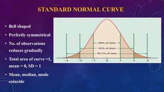
  STANDARD NORMAL CURVE •Bell shaped • Perfectly symmetrical • No. of observations reduces gradually • Total area of curve =1, mean = 0, SD = 1 • Mean, median, mode coincide
• 52.
  EMPIRICAL RULE • Thearea between one standard deviation on either side of the mean will include approximately 68% of the values • The area between two standard deviation on either side of the mean will include approximately 95% of the values • The area between three standard deviation on either side of the mean will include approximately 99.7% of the values
• 53.
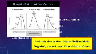
  SKEWNESS • Skewness isthe measure of asymmetry of the distribution • Positive skewness indicates a long right tail • Negative skewness indicates a long left tail • Zero skewness indicates a symmetry around the mean Positively skewed data: Mean>Median>Mode Negatively skewed data: Mean<Median<Mode
• 54.
  TESTS OF SIGNIFICANCE Statisticalprocedures to draw inferences from samples about population Why required? Whether difference between sample estimate and population values is significant or not? Differences between different sample estimates significant or not?
• 55.
  STEPS IN TESTSOF SIGNIFICANCE State Null Hypothesis clearly (Ho) Choose Level of Significance (α) Decide test of Significance Calculate value of test statistic Obtain P-Value and Conclude Ho
• 56.
  • According toRobson (1994), a parametric statistical test is a test whose model specifies certain conditions about the parameters of the population from which the research sample was drawn. PARAMETRIC TESTS
• 57.
  • Parametric testsare more robust and require less data to make a stronger conclusion To use a parametric test, • Data need to be normally distributed, • Data also need to have equal variance and have the same standard deviation. • Continuous Data
• 58.
  PARAMETRIC TESTS 1. PearsonProduct Correlation Coefficient test 2. T test 3. Z test 4. ANOVA
• 59.
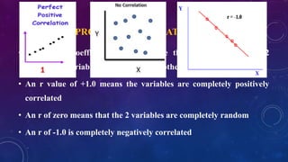
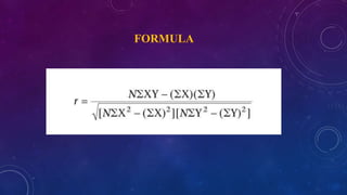
  PEARSON PRODUCT CORRELATIONCOEFFICIENT • Correlation coefficient (r) is a value that tells us how well 2 continuous variables correlate to each other. • An r value of +1.0 means the variables are completely positively correlated • An r of zero means that the 2 variables are completely random • An r of -1.0 is completely negatively correlated
• 60.
  FORMULA
• 61.
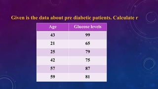
  Given is thedata about pre diabetic patients. Calculate r Age Glucose levels 43 99 21 65 25 79 42 75 57 87 59 81
• 62.
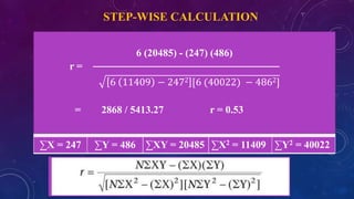
  STEP-WISE CALCULATION X Y 4399 21 65 25 79 42 75 57 87 59 81 X * Y 4257 1365 1975 3150 4959 4779 X2 1849 441 625 1764 3249 3481 Y2 9801 4225 6241 5625 7569 6561 ∑X = 247 ∑Y = 486 ∑XY = 20485 ∑X2 = 11409 ∑Y2 = 40022 6 (20485) - (247) (486) 6 11409 − 2472 [6 (40022) − 4862] r = = 2868 / 5413.27 r = 0.53
• 63.
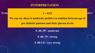
  INTERPRETATION Evans (1996) suggestedthe strength of correlation for the absolute value of r: 0.00-.19 - very weak 0.20-.39 - weak 0 .40-.59 - moderate 0 .60-.79 - strong 0 .80-1.0 - very strong r = 0.53 We can say there is moderate positive co-relation between age of pre diabetic patients and their glucose levels
• 64.
  Z- TEST • Az-test is used for testing the mean of a sample versus population mean, or comparing the means of two populations, with large (n ≥ 30) samples • It is also used for testing the proportion of some characteristic versus a standard proportion, or comparing the proportions of two populations. 64
• 65.
  65 A principal ata certain school claims that the students in his school have above average intelligence. A random sample of 30 students IQ scores have a mean score of 112. Is there sufficient evidence to support the principal’s claim? The mean population IQ is 100 with a standard deviation of 15. Step 1: State the null hypothesis. The accepted fact is that the population mean is 100, so: H0 is μ = 100 Step 2: State the alternate hypothesis. The claim is that the students have above average IQ scores, so H1 is μ > 100.
• 66.
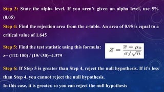
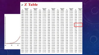
  Step 3: Statethe alpha level. If you aren’t given an alpha level, use 5% (0.05) Step 4: Find the rejection area from the z-table. An area of 0.95 is equal to a critical value of 1.645 Step 5: Find the test statistic using this formula: z= (112-100) / (15/√30)=4.379 Step 6: If Step 5 is greater than Step 4, reject the null hypothesis. If it’s less than Step 4, you cannot reject the null hypothesis. In this case, it is greater, so you can reject the null hypothesis
• 67.
  Total area =0.95 CRITICAL VALUE 0.5 0.5 – 0.05 = 0.45
• 68.
  T- TEST Derived byWilliam Seally Gosset in 1908 Assumption for t test: i. Standard deviation is not known ii. n < 30 iii. Data must be quantitative 68
• 69.
  Types of ttest: a. Paired t test b. Unpaired t test 69
• 70.
  Paired t test: •Consists of a sample of matched pairs of similar units, or one group of units that has been tested twice (a "repeated measures" t-test). • Ex. where subjects are tested prior to a treatment, say for probing depth, and the same subjects are tested again after treatment 70
• 71.
  • Suppose asample of n students were given a diagnostic test before studying a particular module and then again after completing the module. Find out if, teaching leads to improvements in students’ test scores. • Let x = test score before the module and Y= test score after the module • Null hypothesis : true mean difference is zero • Calculate the difference (di = yi − xi) between the two observations on each pair
• 72.
  • Calculate themean difference, d. • Calculate the standard deviation of the differences, Sd, and use this to calculate the Standard error of the mean difference, SEd = Sd/√n • Calculate the t-statistic, which is given by T = d/ SEd • Under the null hypothesis, this statistic follows a t-distribution with n − 1 degrees of freedom. • Use tables of the t-distribution to compare your value for t to the n−1 distribution.
• 73.
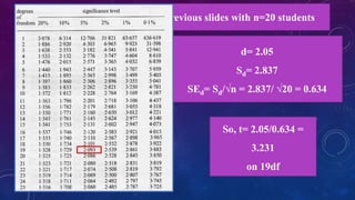
  Using the stepsmentioned in previous slides with n=20 students d= 2.05 Sd= 2.837 SEd= Sd/√n = 2.837/ √20 = 0.634 So, t= 2.05/0.634 = 3.231 on 19df
• 74.
  Unpaired t test: •When two separate sets of independent and identically distributed samples are obtained, one from each of the two populations being compared. • Ex: 1. compare the height of girls and boys. 2. compare 2 stress reduction interventions when one group practiced mindfulness meditation while the other learned progressive muscle relaxation. 74
• 77.
  ANALYSIS OF VARIANCE(ANOVA) •Analysis of variance (ANOVA) is a collection of statistical models used to analyze the differences between group means (such as "variation" among and between groups) • Compares multiple groups at one time • Developed by R.A. Fisher. 77
• 78.
  NON PARAMETRIC TESTS •If data doesn't meet the criteria for a parametric test • Requires more data • Distribution free, easy to calculate • Less efficient
• 79.
  NON PARAMETRIC TESTS •Commonly used Non Parametric Tests are: − Chi Square test − McNemar test − Wilcoxon Signed-Ranks Test − Mann–Whitney U test − Kruskal Wallis test − Friedman test
• 80.
  CHI SQUARE TEST •First used by Karl Pearson • Simplest & most widely used non-parametric test • Calculated using the formula- χ2 = ∑ ( O – E )2 E O = observed frequencies E = expected frequencies Karl Pearson (1857–1936)
• 81.
  STEPS IN THECALCULATION 1. Test the null hypothesis 2. Calculating chi square statistic 3. Applying chi square test 4. Finding degree of freedom 5. Probability tables
• 82.
  • Application ofchi-square test: • Test of association (smoking & cancer, treatment & outcome of disease, vaccination & immunity) • Test of proportions (compare frequencies of diabetics & non- diabetics in groups weighing 40-50kg, 50-60kg, 60-70kg & >70kg.) • The chi-square for goodness of fit (determine if actual numbers are similar to the expected/theoretical numbers)
• 83.
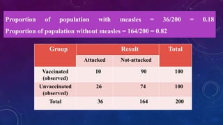
  • Attack ratesamong vaccinated & unvaccinated children against measles • Prove protective value of vaccination by χ2 test at 5% level of significance Group Result Total Attacked Not-attacked Vaccinated (observed) 10 90 100 Unvaccinated (observed) 26 74 100 Total 36 164 200 Proportion of population with measles = 36/200 = 0.18 Proportion of population without measles = 164/200 = 0.82
• 84.
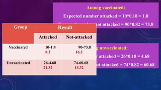
  Among unvaccinated: Expected numberattacked = 26*0.18 = 4.68 Expected number not attacked = 74*0.82 = 60.68 Among vaccinated: Expected number attacked = 10*0.18 = 1.8 Expected number not attacked = 90*0.82 = 73.8 Group Result Attacked Not-attacked Vaccinated 10-1.8 8.2 90-73.8 16.2 Unvaccinated 26-4.68 21.32 74-60.68 13.32
• 85.
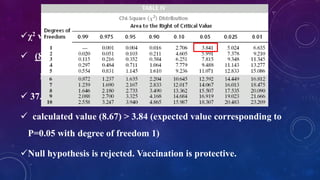
  χ2 value =∑ (O-E)2/E  (8.2)2 + (16.2)2 + (21.32)2 + (13.32)2 1.8 73.8 4.68 60.68  37.35 + 3.5561 + 97.12 + 2.923 = 140.949  calculated value (8.67) > 3.84 (expected value corresponding to P=0.05 with degree of freedom 1) Null hypothesis is rejected. Vaccination is protective.
• 86.
  FISHER’S EXACT TEST •Used when the • Total number of cases is <20 or • The expected number of cases in any cell is ≤1 or • More than 25% of the cells have expected frequencies <5. Ronald A. Fisher (1890–1962)
• 87.
  Mc NEMAR TEST •Used to compare before and after findings in the same individual or to compare findings in a matched analysis • Example: comparing the attitudes of medical students toward confidence in statistics analysis before and after the intensive statistics course. McNemar
• 88.
  88 WILCOXON SIGNED-RANK TEST •Nonparametric equivalent of the paired t-test. • Takes into consideration the magnitude of difference among the pairs of values. WILCOXON
• 89.
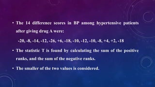
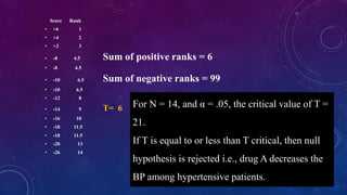
  • The 14difference scores in BP among hypertensive patients after giving drug A were: -20, -8, -14, -12, -26, +6, -18, -10, -12, -10, -8, +4, +2, -18 • The statistic T is found by calculating the sum of the positive ranks, and the sum of the negative ranks. • The smaller of the two values is considered.
• 90.
  Score Rank • +61 • +4 2 • +2 3 • -8 4.5 Sum of positive ranks = 6 • -8 4.5 • -10 6.5 Sum of negative ranks = 99 • -10 6.5 • -12 8 • -14 9 T= 6 • -16 10 • -18 11.5 • -18 11.5 • -20 13 • -26 14 For N = 14, and α = .05, the critical value of T = 21. If T is equal to or less than T critical, then null hypothesis is rejected i.e., drug A decreases the BP among hypertensive patients.
• 91.
  MANN-WHITNEY U TEST •Mann-Whitney U – similar to Wilcoxon signed-ranks test except that the samples are independent and not paired • Null hypothesis: the population means are the same for the two groups • Rank the combined data values for the two groups. Then find the average rank in each group.
• 92.
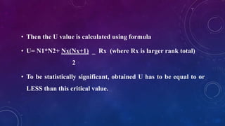
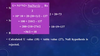
  • Then theU value is calculated using formula • U= N1*N2+ Nx(Nx+1) _ Rx (where Rx is larger rank total) 2 • To be statistically significant, obtained U has to be equal to or LESS than this critical value.
• 93.
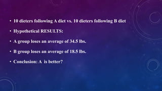
  • 10 dietersfollowing A diet vs. 10 dieters following B diet • Hypothetical RESULTS: • A group loses an average of 34.5 lbs. • B group loses an average of 18.5 lbs. • Conclusion: A is better?
• 94.
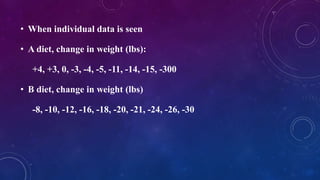
  • When individualdata is seen • A diet, change in weight (lbs): +4, +3, 0, -3, -4, -5, -11, -14, -15, -300 • B diet, change in weight (lbs) -8, -10, -12, -16, -18, -20, -21, -24, -26, -30
• 95.
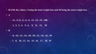
  • RANK thevalues, 1 being the least weight loss and 20 being the most weight loss. • A – +4, +3, 0, -3, -4, -5, -11, -14, -15, -300 – 1, 2, 3, 4, 5, 6, 9, 11, 12, 20 • B − -8, -10, -12, -16, -18, -20, -21, -24, -26, -30 − 7, 8, 10, 13, 14, 15, 16, 17, 18, 19
• 96.
  • Sum ofA’s ranks: 1+ 2 + 3 + 4 + 5 + 6 + 9 + 11+ 12 + 20=73 • Sum of B’s ranks: 7 + 8 +10+ 13+ 14+ 15+16+ 17+ 18+19=137 • B clearly ranked higher. • Calculated U value (18) < table value (27), Null hypothesis is rejected. U= N1*N2+ Nx(Nx+1) _ Rx 2 = 10* 10 + 20 (20+1)/2 – 137 = 100 + 210/2 – 137 = 200+210+274/2 =36/2 = 18
• 97.
  KRUSKAL-WALLIS • It’s morepowerful than Chi-square test. • It is computed exactly like the Mann-Whitney test, except that there are more groups (>2 groups).
• 98.
  FRIEDMAN TEST • Friedman: When either a matched-subjects or repeated- measure design is used and the hypothesis of a difference among three or more (k) treatments is to be tested, the Friedman ANOVA can be used.
• 99.
  SPEARMAN CORRELATION COEFFICIENTTEST • Spearman correlation coefficient, rs, can take values from +1 to -1. • A rs of +1 indicates a perfect association of ranks, a rs of zero indicates no association between ranks and a rs of -1 indicates a perfect negative association of ranks.
• 100.
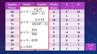
  S English Marks Maths Marks 56 66 75 70 4540 71 60 62 65 64 56 58 59 80 77 76 67 61 63 English Rank Maths Rank 9 4 3 2 10 10 4 7 6 5 5 9 8 8 1 1 2 3 7 6 d d2 5 25 1 1 0 0 -3 9 1 1 -4 16 0 0 0 0 -1 1 1 1 ∑ d2 54