Download as PDF, PPTX


![Confidence interval with quantiles
Suppose we have a sample of data from an exponential distribution
with parameter λ:
f (x|λ) = λe−λx (remember: the estimation of λ is
ˆλ = 1/ˆxn).
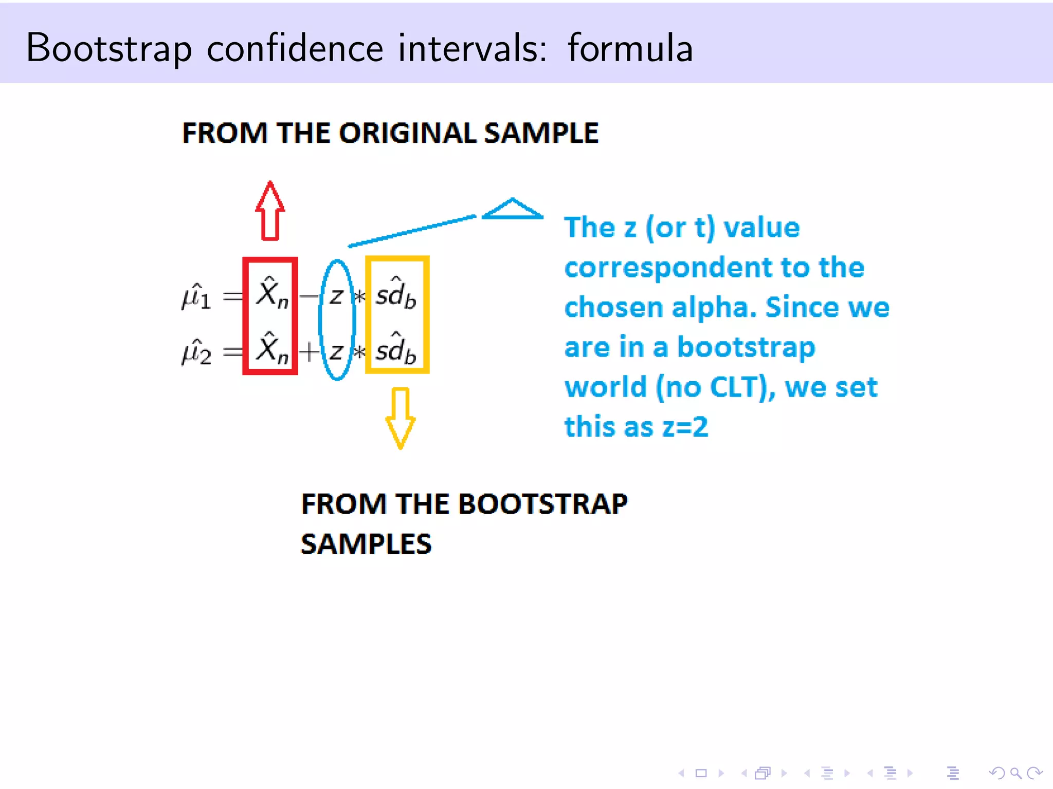
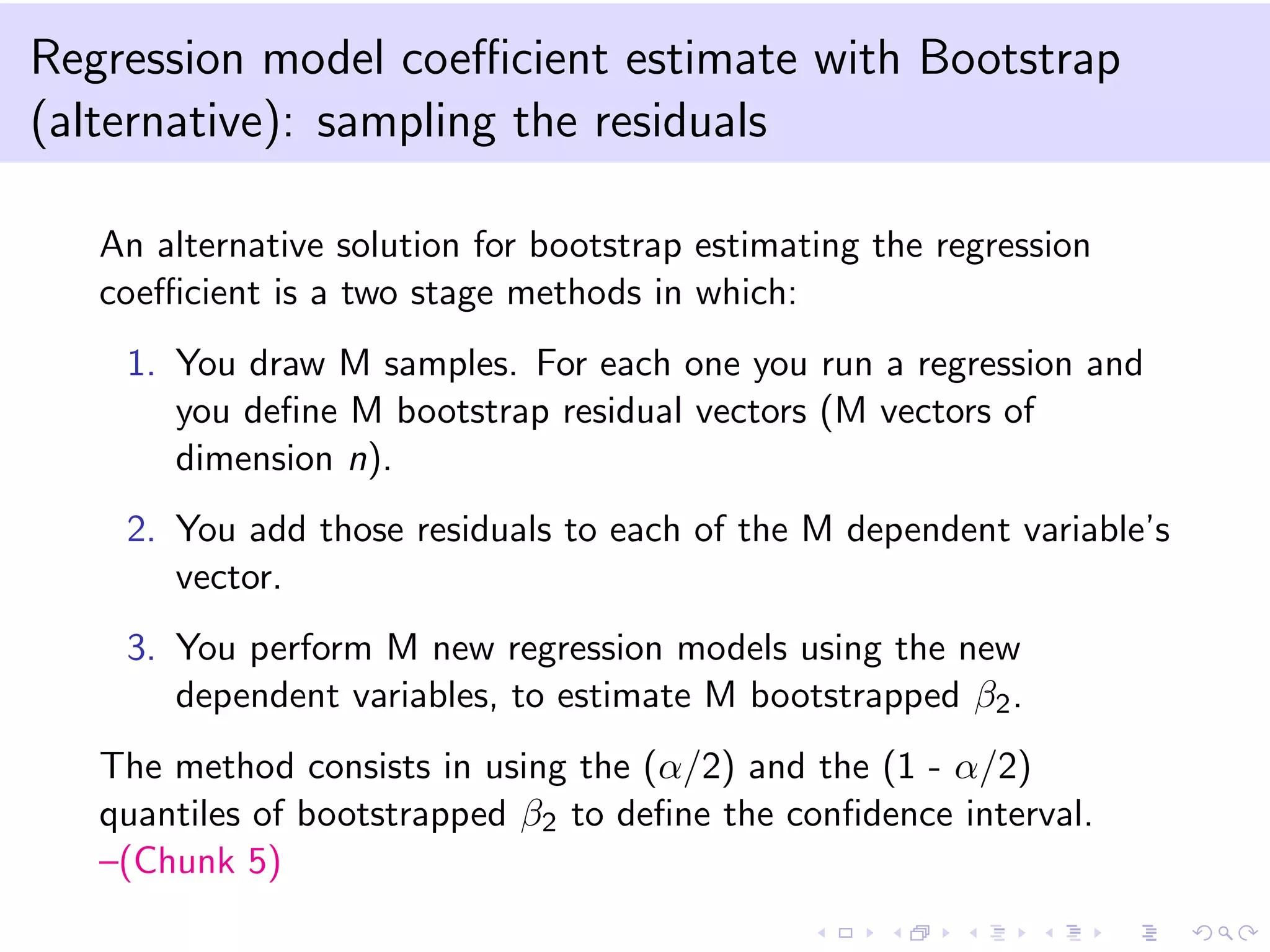
An alternative solution to the use of bootstrap estimated standard
errors (since the estimation of the standard errors from an
exponential is not straightforward) is the use of bootstrap
quantiles.
We can obtain M bootstrap estimates ˆλb and define q∗(α) the α
quantile of the bootstrap distribution of the M λ estimates.
The new bootstrap confidence interval for λ will be:
[2 ∗ ˆλ − q∗(1 − α/2); 2 ∗ ˆλ − q∗(α/2)] –(Chunk 3)](https://image.slidesharecdn.com/talk5-150127122032-conversion-gate02/75/Talk-5-10-2048.jpg)


![Notation
We define a stochastic process {Xt, t = 0, 1, 2, ...} that takes on a
finite or countable number of possible values.
Let the possible values be non negative integers (i.e.Xt ∈ Z+). If
Xt = i, then the process is said to be in state i at time t.
The Markov process (in discrete time) is defined as follows:
Pij = P[Xt+1 = j|Xt = i, Xt−1 = i, ..., X0 = i] = P[Xt+1 = j|Xt =
i], ∀i, j ∈ Z+
We call Pij a 1-step transition probability because we move from
time t to time t + 1.
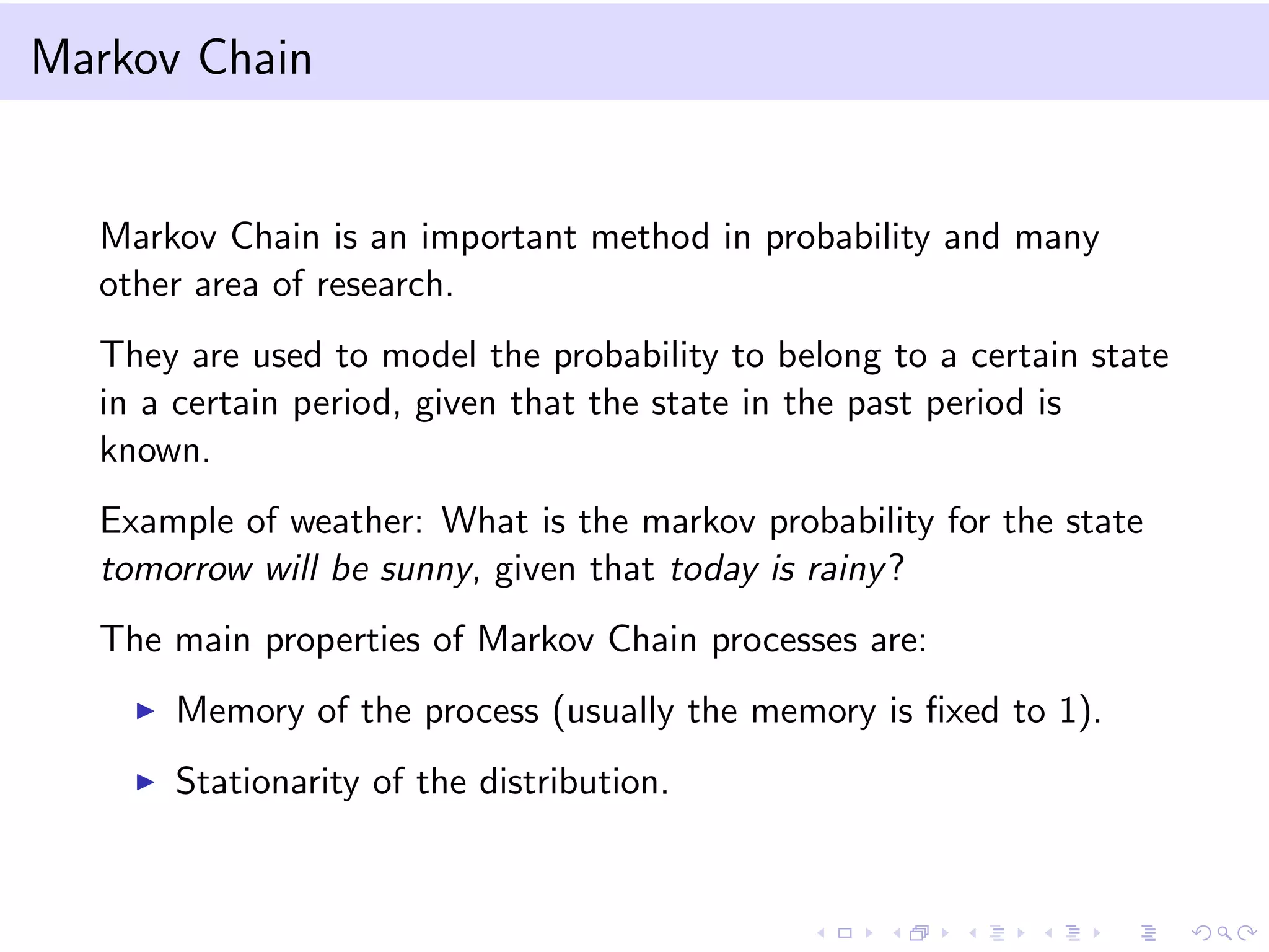
It is a first order Markov Chain (memory = 1) because the
probability of being in state j at time (t + 1) only depends on the
state at time t.](https://image.slidesharecdn.com/talk5-150127122032-conversion-gate02/75/Talk-5-17-2048.jpg)
![Notation - 2
The t − step transition probability
Ptij = P[Xt+k = j|Xk = i], ∀t ≥ 0, i, j ≥ 0
The Champman Kolmogorov equations allow us to compute these
t − step transition probabilities. It states that:
Ptij = k PtikPmkj , ∀t, m ≥ 0, ∀i, j ≥ 0
N.B. Base probability properties:
1. Pij ≥ 0, ∀i, j ≥ 0
2. j≥0 Pij = 1, i = 0, 1, 2, ...](https://image.slidesharecdn.com/talk5-150127122032-conversion-gate02/75/Talk-5-18-2048.jpg)
![Example: conditional probability
Consider two states: 0 = rain and 1 = no rain.
Define two probabilities:
α = P00 = P[Xt+1 = 0|Xt = 0] the probability it will rain
tomorrow given it rains today
β = P01 = P[Xt+1 = 1|Xt = 0] the probability it will rain
tomorrow given it does not rain today. What is the probability it
will rain the day after tomorrow given it rains today, given α = 0.7
and β = 0.3?
The transition probability matrix will be:
P = [P00, P01, P10, P11], or
P = [α = 0.7, β = 0.3, 1 − α = 0.4, 1 − β = 0.6] –(Chunk 6)](https://image.slidesharecdn.com/talk5-150127122032-conversion-gate02/75/Talk-5-19-2048.jpg)
![Example: unconditional probababily
What is the unconditional probability it will rain the day after
tomorrow?
We need to define the unconditional or marginal distribution of the
state at time t:
P[Xt = j] = i P[Xt = j|X0 = 1]P[X0 = i] = i Ptij ∗ αi ,
where αi = P[X0 = i], ∀i ≥ 0
and P[Xt = j|X0 = 1] is the conditional probability just computed
before. –(Chunk 7)](https://image.slidesharecdn.com/talk5-150127122032-conversion-gate02/75/Talk-5-20-2048.jpg)


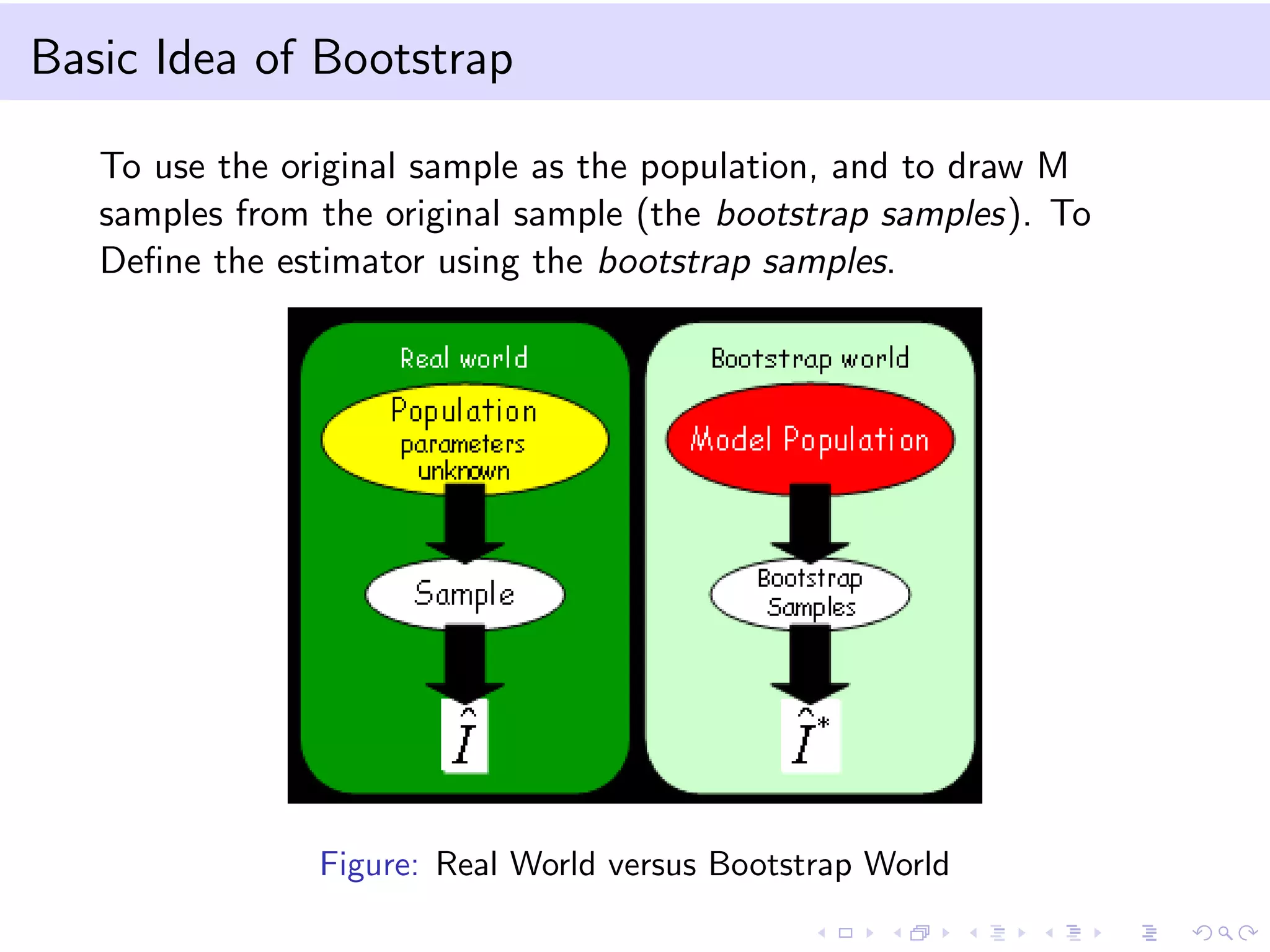
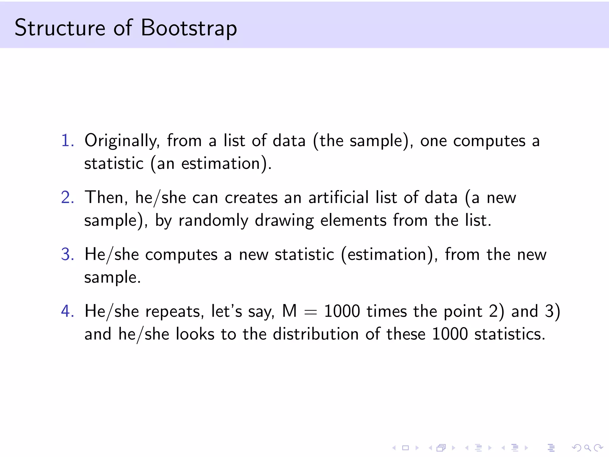
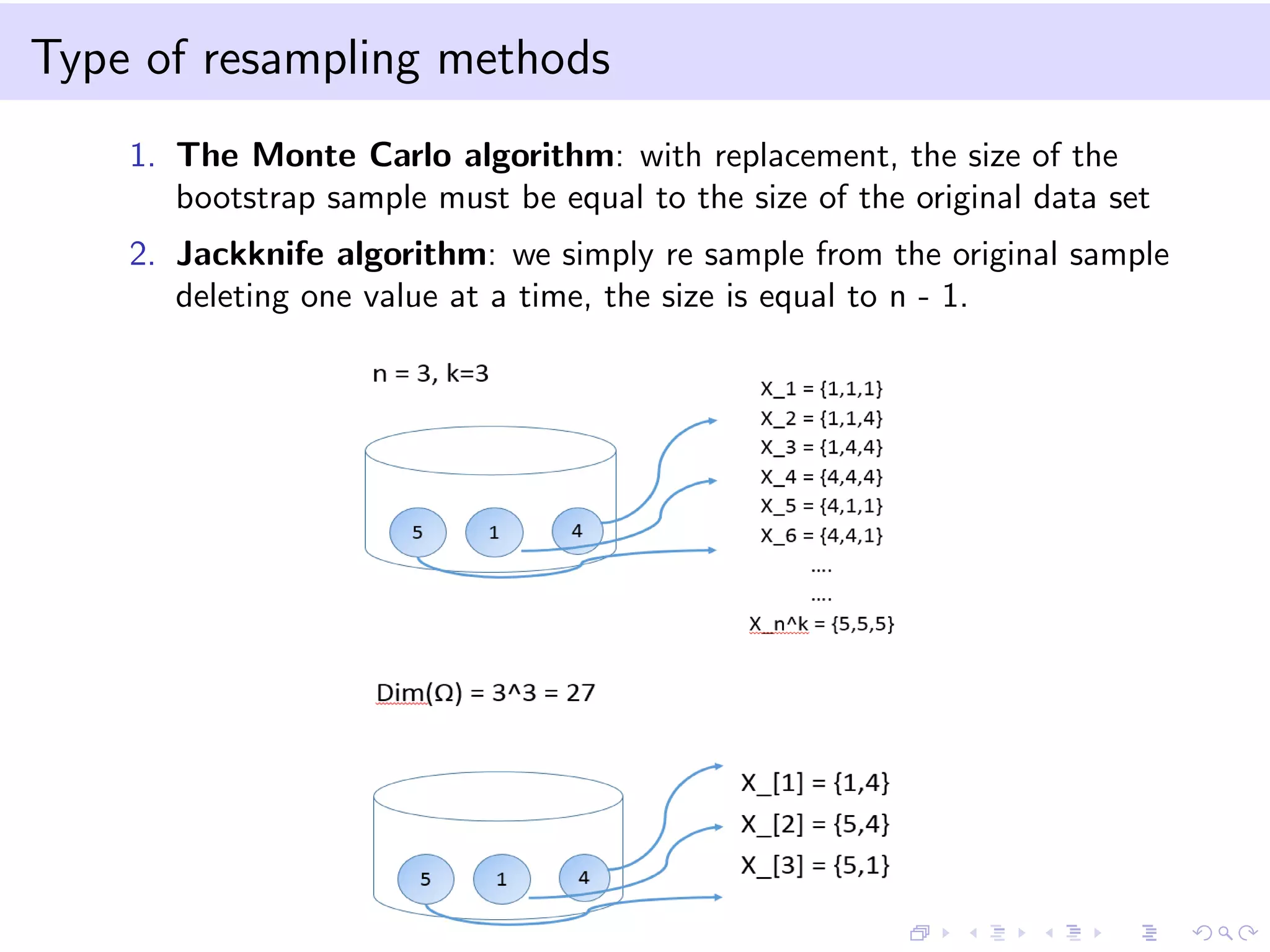
The document provides an introduction to bootstrap resampling methods and Markov chains. It explains the bootstrap technique for estimating the sampling distribution and variance of estimators when sample sizes are small, using resampling from the original sample, and derives confidence intervals based on bootstrapped estimates. The Markov chain section details the properties and definitions of Markov processes, including transition probabilities and stationary distributions.