Download as PDF, PPTX


![Markov Chain Monte Carlo Methods
New [2004] edition:](https://image.slidesharecdn.com/main-091109121752-phpapp01/85/Monte-Carlo-Statistical-Methods-3-320.jpg?cb=1713217764)


![Markov Chain Monte Carlo Methods
Motivation and leading example
Missing variable models
The EM Algorithm
Gibbs connection Bayes rather than EM
Algorithm (Expectation–Maximisation)
Iterate (in m)
1. (E step) Compute
ˆ ˆ
Q(θ|θ(m) , x) = E[log Lc (θ|x, Z)|θ(m) , x] ,](https://image.slidesharecdn.com/main-091109121752-phpapp01/85/Monte-Carlo-Statistical-Methods-21-320.jpg?cb=1713217764)
![Markov Chain Monte Carlo Methods
Motivation and leading example
Missing variable models
The EM Algorithm
Gibbs connection Bayes rather than EM
Algorithm (Expectation–Maximisation)
Iterate (in m)
1. (E step) Compute
ˆ ˆ
Q(θ|θ(m) , x) = E[log Lc (θ|x, Z)|θ(m) , x] ,
ˆ
2. (M step) Maximise Q(θ|θ(m) , x) in θ and take
ˆ ˆ
θ(m+1) = arg max Q(θ|θ(m) , x).
θ
until a fixed point [of Q] is reached](https://image.slidesharecdn.com/main-091109121752-phpapp01/85/Monte-Carlo-Statistical-Methods-22-320.jpg?cb=1713217764)


![Markov Chain Monte Carlo Methods
Motivation and leading example
Bayesian Methods
Central tool
Summary in a probability distribution, π(θ|x), called the posterior
distribution
Derived from the joint distribution f (x|θ)π(θ), according to
f (x|θ)π(θ)
π(θ|x) = ,
f (x|θ)π(θ)dθ
[Bayes Theorem]](https://image.slidesharecdn.com/main-091109121752-phpapp01/85/Monte-Carlo-Statistical-Methods-28-320.jpg?cb=1713217764)
![Markov Chain Monte Carlo Methods
Motivation and leading example
Bayesian Methods
Central tool
Summary in a probability distribution, π(θ|x), called the posterior
distribution
Derived from the joint distribution f (x|θ)π(θ), according to
f (x|θ)π(θ)
π(θ|x) = ,
f (x|θ)π(θ)dθ
[Bayes Theorem]
where
m(x) = f (x|θ)π(θ)dθ
is the marginal density of X](https://image.slidesharecdn.com/main-091109121752-phpapp01/85/Monte-Carlo-Statistical-Methods-29-320.jpg?cb=1713217764)


![Markov Chain Monte Carlo Methods
Motivation and leading example
Bayesian troubles
Example (Mixture once again)
Bayes estimator of θ:
n
δ π (x1 , . . . , xn ) = ω(kt )Eπ [θ|x, (kt )]
ℓ=0 (kt )
Too costly: 2n terms](https://image.slidesharecdn.com/main-091109121752-phpapp01/85/Monte-Carlo-Statistical-Methods-52-320.jpg?cb=1713217764)

![Markov Chain Monte Carlo Methods
Motivation and leading example
Bayesian troubles
Example (Poly-t priors (2))
More involved prior distribution:
poly-t distribution
[Bauwens,1985]
k
−νi
π(θ) = αi + (θ − βi )2 αi , νi > 0
i=1](https://image.slidesharecdn.com/main-091109121752-phpapp01/85/Monte-Carlo-Statistical-Methods-54-320.jpg?cb=1713217764)
![Markov Chain Monte Carlo Methods
Motivation and leading example
Bayesian troubles
Example (Poly-t priors (2))
More involved prior distribution:
poly-t distribution
[Bauwens,1985]
k
−νi
π(θ) = αi + (θ − βi )2 αi , νi > 0
i=1
Computation of E[θ|x] ???](https://image.slidesharecdn.com/main-091109121752-phpapp01/85/Monte-Carlo-Statistical-Methods-55-320.jpg?cb=1713217764)


![Markov Chain Monte Carlo Methods
Random variable generation
Basic methods
The inverse transform method
For a function F on R, the generalized inverse of F , F − , is defined
by
F − (u) = inf {x; F (x) ≥ u} .
Definition (Probability Integral Transform)
If U ∼ U[0,1] , then the random variable F − (U ) has the distribution
F.](https://image.slidesharecdn.com/main-091109121752-phpapp01/85/Monte-Carlo-Statistical-Methods-64-320.jpg?cb=1713217764)
![Markov Chain Monte Carlo Methods
Random variable generation
Basic methods
The inverse transform method (2)
To generate a random variable X ∼ F , simply generate
U ∼ U[0,1]](https://image.slidesharecdn.com/main-091109121752-phpapp01/85/Monte-Carlo-Statistical-Methods-65-320.jpg?cb=1713217764)
![Markov Chain Monte Carlo Methods
Random variable generation
Basic methods
The inverse transform method (2)
To generate a random variable X ∼ F , simply generate
U ∼ U[0,1]
and then make the transform
x = F − (u)](https://image.slidesharecdn.com/main-091109121752-phpapp01/85/Monte-Carlo-Statistical-Methods-66-320.jpg?cb=1713217764)
![Markov Chain Monte Carlo Methods
Random variable generation
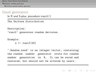
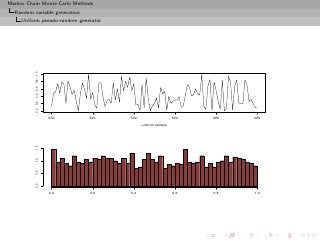
Uniform pseudo-random generator
Desiderata and limitations
skip Uniform
• Production of a deterministic sequence of values in [0, 1] which
imitates a sequence of iid uniform random variables U[0,1] .](https://image.slidesharecdn.com/main-091109121752-phpapp01/85/Monte-Carlo-Statistical-Methods-67-320.jpg?cb=1713217764)
![Markov Chain Monte Carlo Methods
Random variable generation
Uniform pseudo-random generator
Desiderata and limitations
skip Uniform
• Production of a deterministic sequence of values in [0, 1] which
imitates a sequence of iid uniform random variables U[0,1] .
• Can’t use the physical imitation of a “random draw” [no
guarantee of uniformity, no reproducibility]](https://image.slidesharecdn.com/main-091109121752-phpapp01/85/Monte-Carlo-Statistical-Methods-68-320.jpg?cb=1713217764)
![Markov Chain Monte Carlo Methods
Random variable generation
Uniform pseudo-random generator
Desiderata and limitations
skip Uniform
• Production of a deterministic sequence of values in [0, 1] which
imitates a sequence of iid uniform random variables U[0,1] .
• Can’t use the physical imitation of a “random draw” [no
guarantee of uniformity, no reproducibility]
• Random sequence in the sense: Having generated
(X1 , · · · , Xn ), knowledge of Xn [or of (X1 , · · · , Xn )] imparts
no discernible knowledge of the value of Xn+1 .](https://image.slidesharecdn.com/main-091109121752-phpapp01/85/Monte-Carlo-Statistical-Methods-69-320.jpg?cb=1713217764)
![Markov Chain Monte Carlo Methods
Random variable generation
Uniform pseudo-random generator
Desiderata and limitations
skip Uniform
• Production of a deterministic sequence of values in [0, 1] which
imitates a sequence of iid uniform random variables U[0,1] .
• Can’t use the physical imitation of a “random draw” [no
guarantee of uniformity, no reproducibility]
• Random sequence in the sense: Having generated
(X1 , · · · , Xn ), knowledge of Xn [or of (X1 , · · · , Xn )] imparts
no discernible knowledge of the value of Xn+1 .
• Deterministic: Given the initial value X0 , sample
(X1 , · · · , Xn ) always the same](https://image.slidesharecdn.com/main-091109121752-phpapp01/85/Monte-Carlo-Statistical-Methods-70-320.jpg?cb=1713217764)
![Markov Chain Monte Carlo Methods
Random variable generation
Uniform pseudo-random generator
Desiderata and limitations
skip Uniform
• Production of a deterministic sequence of values in [0, 1] which
imitates a sequence of iid uniform random variables U[0,1] .
• Can’t use the physical imitation of a “random draw” [no
guarantee of uniformity, no reproducibility]
• Random sequence in the sense: Having generated
(X1 , · · · , Xn ), knowledge of Xn [or of (X1 , · · · , Xn )] imparts
no discernible knowledge of the value of Xn+1 .
• Deterministic: Given the initial value X0 , sample
(X1 , · · · , Xn ) always the same
• Validity of a random number generator based on a single
sample X1 , · · · , Xn when n tends to +∞, not on replications
(X11 , · · · , X1n ), (X21 , · · · , X2n ), . . . (Xk1 , · · · , Xkn )
where n fixed and k tends to infinity.](https://image.slidesharecdn.com/main-091109121752-phpapp01/85/Monte-Carlo-Statistical-Methods-71-320.jpg?cb=1713217764)
![Markov Chain Monte Carlo Methods
Random variable generation
Uniform pseudo-random generator
Uniform pseudo-random generator
Algorithm starting from an initial value 0 ≤ u0 ≤ 1 and a
transformation D, which produces a sequence
(ui ) = (Di (u0 ))
in [0, 1].](https://image.slidesharecdn.com/main-091109121752-phpapp01/85/Monte-Carlo-Statistical-Methods-72-320.jpg?cb=1713217764)
![Markov Chain Monte Carlo Methods
Random variable generation
Uniform pseudo-random generator
Uniform pseudo-random generator
Algorithm starting from an initial value 0 ≤ u0 ≤ 1 and a
transformation D, which produces a sequence
(ui ) = (Di (u0 ))
in [0, 1].
For all n,
(u1 , · · · , un )
reproduces the behavior of an iid U[0,1] sample (V1 , · · · , Vn ) when
compared through usual tests](https://image.slidesharecdn.com/main-091109121752-phpapp01/85/Monte-Carlo-Statistical-Methods-73-320.jpg?cb=1713217764)
![Markov Chain Monte Carlo Methods
Random variable generation
Uniform pseudo-random generator
Uniform pseudo-random generator (2)
• Validity means the sequence U1 , · · · , Un leads to accept the
hypothesis
H : U1 , · · · , Un are iid U[0,1] .](https://image.slidesharecdn.com/main-091109121752-phpapp01/85/Monte-Carlo-Statistical-Methods-74-320.jpg?cb=1713217764)
![Markov Chain Monte Carlo Methods
Random variable generation
Uniform pseudo-random generator
Uniform pseudo-random generator (2)
• Validity means the sequence U1 , · · · , Un leads to accept the
hypothesis
H : U1 , · · · , Un are iid U[0,1] .
• The set of tests used is generally of some consequence
◦ Kolmogorov–Smirnov and other nonparametric tests
◦ Time series methods, for correlation between Ui and
(Ui−1 , · · · , Ui−k )
◦ Marsaglia’s battery of tests called Die Hard (!)](https://image.slidesharecdn.com/main-091109121752-phpapp01/85/Monte-Carlo-Statistical-Methods-75-320.jpg?cb=1713217764)


![Markov Chain Monte Carlo Methods
Random variable generation
Transformation methods
Transformation methods
Case where a distribution F is linked in a simple way to another
distribution easy to simulate.
Example (Exponential variables)
If U ∼ U[0,1] , the random variable
X = − log U/λ
has distribution
P (X ≤ x) = P (− log U ≤ λx)
= P (U ≥ e−λx ) = 1 − e−λx ,
the exponential distribution E xp(λ).](https://image.slidesharecdn.com/main-091109121752-phpapp01/85/Monte-Carlo-Statistical-Methods-84-320.jpg?cb=1713217764)


![Markov Chain Monte Carlo Methods
Random variable generation
Transformation methods
Box-Muller Algorithm
Example (Normal variables)
If r, θ polar coordinates of (X1 , X2 ), then,
r2 = X1 + X2 ∼ χ2 = E (1/2)
2 2
2 and θ ∼ U [0, 2π]](https://image.slidesharecdn.com/main-091109121752-phpapp01/85/Monte-Carlo-Statistical-Methods-87-320.jpg?cb=1713217764)
![Markov Chain Monte Carlo Methods
Random variable generation
Transformation methods
Box-Muller Algorithm
Example (Normal variables)
If r, θ polar coordinates of (X1 , X2 ), then,
r2 = X1 + X2 ∼ χ2 = E (1/2)
2 2
2 and θ ∼ U [0, 2π]
Consequence: If U1 , U2 iid U[0,1] ,
X1 = −2 log(U1 ) cos(2πU2 )
X2 = −2 log(U1 ) sin(2πU2 )
iid N (0, 1).](https://image.slidesharecdn.com/main-091109121752-phpapp01/85/Monte-Carlo-Statistical-Methods-88-320.jpg?cb=1713217764)
![Markov Chain Monte Carlo Methods
Random variable generation
Transformation methods
Box-Muller Algorithm (2)
1. Generate U1 , U2 iid U[0,1] ;
2. Define
x1 = −2 log(u1 ) cos(2πu2 ) ,
x2 = −2 log(u1 ) sin(2πu2 ) ;
3. Take x1 and x2 as two independent draws from
N (0, 1).](https://image.slidesharecdn.com/main-091109121752-phpapp01/85/Monte-Carlo-Statistical-Methods-89-320.jpg?cb=1713217764)


![Markov Chain Monte Carlo Methods
Random variable generation
Transformation methods
Atkinson’s Poisson
To generate N ∼ P(λ):
1. Define
√
β = π/ 3λ, α = λβ and k = log c−λ−log β;
2. Generate U1 ∼ U[0,1] and calculate
x = {α − log{(1 − u1 )/u1 }}/β
until x > −0.5 ;
3. Define N = ⌊x + 0.5⌋ and generate
U2 ∼ U[0,1] ;
4. Accept N if
α−βx+log (u2 /{1+exp(α−βx)}2 ) ≤ k+N log λ−log N ! .](https://image.slidesharecdn.com/main-091109121752-phpapp01/85/Monte-Carlo-Statistical-Methods-93-320.jpg?cb=1713217764)


![Markov Chain Monte Carlo Methods
Random variable generation
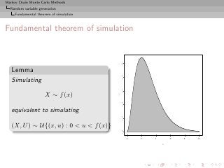
Fundamental theorem of simulation
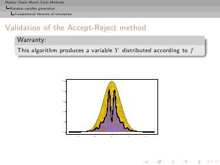
The Accept-Reject algorithm
Given a density of interest f , find a density g and a constant M
such that
f (x) ≤ M g(x)
on the support of f .
1. Generate X ∼ g, U ∼ U[0,1] ;
2. Accept Y = X if U ≤ f (X)/M g(X) ;
3. Return to 1. otherwise.](https://image.slidesharecdn.com/main-091109121752-phpapp01/85/Monte-Carlo-Statistical-Methods-100-320.jpg?cb=1713217764)


![Markov Chain Monte Carlo Methods
Random variable generation
Fundamental theorem of simulation
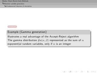
Example (Gamma generation (2))
Can use the Accept-Reject algorithm with instrumental distribution
Ga(a, b), with a = [α], α ≥ 0.
(Without loss of generality, β = 1.)](https://image.slidesharecdn.com/main-091109121752-phpapp01/85/Monte-Carlo-Statistical-Methods-113-320.jpg?cb=1713217764)
![Markov Chain Monte Carlo Methods
Random variable generation
Fundamental theorem of simulation
Example (Gamma generation (2))
Can use the Accept-Reject algorithm with instrumental distribution
Ga(a, b), with a = [α], α ≥ 0.
(Without loss of generality, β = 1.)
Up to a normalizing constant,
α−a
α−a
f /gb = b−a xα−a exp{−(1 − b)x} ≤ b−a
(1 − b)e
for b ≤ 1.
The maximum is attained at b = a/α.](https://image.slidesharecdn.com/main-091109121752-phpapp01/85/Monte-Carlo-Statistical-Methods-114-320.jpg?cb=1713217764)


![Markov Chain Monte Carlo Methods
Random variable generation
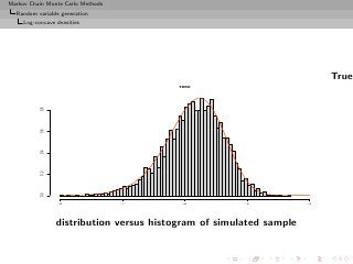
Log-concave densities
Log-concave densities (2)
Take
Sn = {xi , i = 0, 1, . . . , n + 1} ⊂ supp(f )
such that h(xi ) = log f (xi ) known up to the same constant.
By concavity of h, line Li,i+1 through (xi , h(xi )) and
(xi+1 , h(xi+1 ))
◮ below h in [xi , xi+1 ] and
◮ above this graph outside this interval
L 2,3 (x)
log f(x)
x1 x2 x3 x4
x](https://image.slidesharecdn.com/main-091109121752-phpapp01/85/Monte-Carlo-Statistical-Methods-122-320.jpg?cb=1713217764)
![Markov Chain Monte Carlo Methods
Random variable generation
Log-concave densities
Log-concave densities (3)
For x ∈ [xi , xi+1 ], if
hn (x) = min{Li−1,i (x), Li+1,i+2 (x)} and hn (x) = Li,i+1 (x) ,
the envelopes are
hn (x) ≤ h(x) ≤ hn (x)
uniformly on the support of f , with
hn (x) = −∞ and hn (x) = min(L0,1 (x), Ln,n+1 (x))
on [x0 , xn+1 ]c .](https://image.slidesharecdn.com/main-091109121752-phpapp01/85/Monte-Carlo-Statistical-Methods-123-320.jpg?cb=1713217764)

![Markov Chain Monte Carlo Methods
Random variable generation
Log-concave densities
ARS Algorithm
1. Initialize n and Sn .
2. Generate X ∼ gn (x), U ∼ U[0,1] .
3. If U ≤ f n (X)/̟n gn (X), accept X;
otherwise, if U ≤ f (X)/̟n gn (X), accept X](https://image.slidesharecdn.com/main-091109121752-phpapp01/85/Monte-Carlo-Statistical-Methods-125-320.jpg?cb=1713217764)


![Markov Chain Monte Carlo Methods
Random variable generation
Log-concave densities
Example (Northern Pintail ducks (3))
Prior selection
If
N ∼ P(λ)
and
pi
αi = log ∼ N (µi , σ 2 ),
1 − pi
[Normal logistic]](https://image.slidesharecdn.com/main-091109121752-phpapp01/85/Monte-Carlo-Statistical-Methods-128-320.jpg?cb=1713217764)


![Markov Chain Monte Carlo Methods
Monte Carlo Integration
Monte Carlo integration
Monte Carlo integration
Theme:
Generic problem of evaluating the integral
I = Ef [h(X)] = h(x) f (x) dx
X
where X is uni- or multidimensional, f is a closed form, partly
closed form, or implicit density, and h is a function](https://image.slidesharecdn.com/main-091109121752-phpapp01/85/Monte-Carlo-Statistical-Methods-139-320.jpg?cb=1713217764)

![Markov Chain Monte Carlo Methods
Monte Carlo Integration
Monte Carlo integration
Monte Carlo integration (2)
Monte Carlo solution
First use a sample (X1 , . . . , Xm ) from the density f to
approximate the integral I by the empirical average
m
1
hm = h(xj )
m
j=1
which converges
hm −→ Ef [h(X)]
by the Strong Law of Large Numbers](https://image.slidesharecdn.com/main-091109121752-phpapp01/85/Monte-Carlo-Statistical-Methods-141-320.jpg?cb=1713217764)
![Markov Chain Monte Carlo Methods
Monte Carlo Integration
Monte Carlo integration
Monte Carlo precision
Estimate the variance with
m
1 1
vm = [h(xj ) − hm ]2 ,
mm−1
j=1
and for m large,
hm − Ef [h(X)]
√ ∼ N (0, 1).
vm
Note: This can lead to the construction of a convergence test and
of confidence bounds on the approximation of Ef [h(X)].](https://image.slidesharecdn.com/main-091109121752-phpapp01/85/Monte-Carlo-Statistical-Methods-142-320.jpg?cb=1713217764)


![Markov Chain Monte Carlo Methods
Monte Carlo Integration
Importance Sampling
Importance sampling
Paradox
Simulation from f (the true density) is not necessarily optimal
Alternative to direct sampling from f is importance sampling,
based on the alternative representation
f (x)
Ef [h(X)] = h(x) g(x) dx .
X g(x)
which allows us to use other distributions than f](https://image.slidesharecdn.com/main-091109121752-phpapp01/85/Monte-Carlo-Statistical-Methods-147-320.jpg?cb=1713217764)
![Markov Chain Monte Carlo Methods
Monte Carlo Integration
Importance Sampling
Importance sampling algorithm
Evaluation of
Ef [h(X)] = h(x) f (x) dx
X
by
1. Generate a sample X1 , . . . , Xn from a distribution g
2. Use the approximation
m
1 f (Xj )
h(Xj )
m g(Xj )
j=1](https://image.slidesharecdn.com/main-091109121752-phpapp01/85/Monte-Carlo-Statistical-Methods-148-320.jpg?cb=1713217764)

![Markov Chain Monte Carlo Methods
Monte Carlo Integration
Importance Sampling
Same thing as before!!!
Convergence of the estimator
m
1 f (Xj )
h(Xj ) −→ h(x) f (x) dx
m g(Xj ) X
j=1
converges for any choice of the distribution g
[as long as supp(g) ⊃ supp(f )]](https://image.slidesharecdn.com/main-091109121752-phpapp01/85/Monte-Carlo-Statistical-Methods-150-320.jpg?cb=1713217764)


![Markov Chain Monte Carlo Methods
Monte Carlo Integration
Importance Sampling
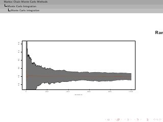
200
150
100
50
0
0 2000 4000 6000 8000 10000
iterations
Range
and average of 500 replications of IS estimate of E[exp −X]
over 10, 000 iterations.](https://image.slidesharecdn.com/main-091109121752-phpapp01/85/Monte-Carlo-Statistical-Methods-156-320.jpg?cb=1713217764)


![Markov Chain Monte Carlo Methods
Monte Carlo Integration
Importance Sampling
Selfnormalised importance sampling
For ratio estimator
n n
n
δh = ωi h(xi ) ωi
i=1 i=1
with Xi ∼ g(y) and Wi such that
E[Wi |Xi = x] = κf (x)/g(x)](https://image.slidesharecdn.com/main-091109121752-phpapp01/85/Monte-Carlo-Statistical-Methods-161-320.jpg?cb=1713217764)
![Markov Chain Monte Carlo Methods
Monte Carlo Integration
Importance Sampling
Selfnormalised variance
then
n 1
var(δh ) ≈ var(Sh ) − 2Eπ [h] cov(Sh , S1 ) + Eπ [h]2 var(S1 ) .
n n n n
n2 κ2
for
n n
n n
Sh = Wi h(Xi ) , S1 = Wi
i=1 i=1
Rough approximation
n 1
varδh ≈ varπ (h(X)) {1 + varg (W )}
n](https://image.slidesharecdn.com/main-091109121752-phpapp01/85/Monte-Carlo-Statistical-Methods-162-320.jpg?cb=1713217764)


![Markov Chain Monte Carlo Methods
Monte Carlo Integration
Importance Sampling
Example (Student’s t distribution (2))
• Simulation possibilities
◦ Directly from fν , since fν = N (0,1)
√ 2
χν
◦ Importance sampling using Cauchy C (0, 1)
◦ Importance sampling using a normal N (0, 1)
(expected to be nonoptimal)
◦ Importance sampling using a U ([0, 1/2.1])
change of variables](https://image.slidesharecdn.com/main-091109121752-phpapp01/85/Monte-Carlo-Statistical-Methods-167-320.jpg?cb=1713217764)
![Markov Chain Monte Carlo Methods
Monte Carlo Integration
Importance Sampling
Sampling
7.0
6.5
6.0
5.5
5.0
0 10000 20000 30000 40000 50000
from f (solid lines), importance sampling with Cauchy
instrumental (short dashes), U ([0, 1/2.1]) instrumental (long
dashes) and normal instrumental (dots).](https://image.slidesharecdn.com/main-091109121752-phpapp01/85/Monte-Carlo-Statistical-Methods-168-320.jpg?cb=1713217764)


![Markov Chain Monte Carlo Methods
Monte Carlo Integration
Importance Sampling
IS suffers (2)
Since E[Vn+1 ] = 1 and Vn+1 independent from Fn ,
E(Un+1 | Fn ) = Un E(Vn+1 | Fn ) = Un ,
and thus {Un }n≥0 martingale
√
Since x → x concave, by Jensen’s inequality,
E( Un+1 | Fn ) ≤ E(Un+1 | Fn ) ≤ Un
√
and thus { Un }n≥0 supermartingale
Assume E( Vn+1 ) < 1. Then
n
E( Un ) = E( Vk ) → 0, n → ∞.
k=1](https://image.slidesharecdn.com/main-091109121752-phpapp01/85/Monte-Carlo-Statistical-Methods-171-320.jpg?cb=1713217764)


![Markov Chain Monte Carlo Methods
Monte Carlo Integration
Acceleration methods
Integration by conditioning
Use Rao-Blackwell Theorem
var(E[δ(X)|Y]) ≤ var(δ(X))](https://image.slidesharecdn.com/main-091109121752-phpapp01/85/Monte-Carlo-Statistical-Methods-191-320.jpg?cb=1713217764)
![Markov Chain Monte Carlo Methods
Monte Carlo Integration
Acceleration methods
Consequence
If I unbiased estimator of I = Ef [h(X)], with X simulated from a
˜
joint density f (x, y), where
˜
f (x, y)dy = f (x),
the estimator
I∗ = Ef [I|Y1 , . . . , Yn ]
˜
dominate I(X1 , . . . , Xn ) variance-wise (and is unbiased)](https://image.slidesharecdn.com/main-091109121752-phpapp01/85/Monte-Carlo-Statistical-Methods-192-320.jpg?cb=1713217764)
![Markov Chain Monte Carlo Methods
Monte Carlo Integration
Acceleration methods
skip expectation
Example (Student’s t expectation)
For
E[h(x)] = E[exp(−x2 )] with X ∼ T (ν, 0, σ 2 )
a Student’s t distribution can be simulated as
X|y ∼ N (µ, σ 2 y) and Y −1 ∼ χ2 .
ν](https://image.slidesharecdn.com/main-091109121752-phpapp01/85/Monte-Carlo-Statistical-Methods-193-320.jpg?cb=1713217764)

![Markov Chain Monte Carlo Methods
Monte Carlo Integration
Acceleration methods
Example (Student’s t expectation (2))
Empirical distribution
m
1 2
exp(−Xj ) ,
m
j=1
can be improved from the joint sample
((X1 , Y1 ), . . . , (Xm , Ym ))
since
m m
1 1 1
E[exp(−X 2 )|Yj ] =
m m 2σ 2 Yj + 1
j=1 j=1
is the conditional expectation.
In this example, precision ten times better](https://image.slidesharecdn.com/main-091109121752-phpapp01/85/Monte-Carlo-Statistical-Methods-195-320.jpg?cb=1713217764)
![Markov Chain Monte Carlo Methods
Monte Carlo Integration
Acceleration methods
Estimators
0.60
0.58
0.56
0.54
0.52
0.50
0 2000 4000 6000 8000 10000
of E[exp(−X 2 )]: empirical average (full) and conditional
expectation (dotted) for (ν, µ, σ) = (4.6, 0, 1).](https://image.slidesharecdn.com/main-091109121752-phpapp01/85/Monte-Carlo-Statistical-Methods-196-320.jpg?cb=1713217764)


![Markov Chain Monte Carlo Methods
Monte Carlo Integration
Bayesian importance sampling
g(θ) = ρπ(θ) + (1 − ρ)π(θ|x)
♦ defensive mixture
♦ ρ ≪ 1 Ok
[Hestenberg, 1998]](https://image.slidesharecdn.com/main-091109121752-phpapp01/85/Monte-Carlo-Statistical-Methods-200-320.jpg?cb=1713217764)
![Markov Chain Monte Carlo Methods
Monte Carlo Integration
Bayesian importance sampling
g(θ) = ρπ(θ) + (1 − ρ)π(θ|x)
♦ defensive mixture
♦ ρ ≪ 1 Ok
[Hestenberg, 1998]
g(θ) = π(θ|x)
1
♦ mh (x) = T
1 h(θ)
T t=1 f (x|θ)π(θ)
♦ works for any h
♦ finite variance if
h2 (θ)
dθ < ∞
f (x|θ)π(θ)](https://image.slidesharecdn.com/main-091109121752-phpapp01/85/Monte-Carlo-Statistical-Methods-201-320.jpg?cb=1713217764)
![Markov Chain Monte Carlo Methods
Monte Carlo Integration
Bayesian importance sampling
Bridge sampling
[Chen & Shao, 1997]
Given two models f1 (x|θ1 ) and f2 (x|θ2 ),
π1 (θ1 )f1 (x|θ1 )
π1 (θ1 |x) =
m1 (x)
π2 (θ2 )f2 (x|θ2 )
π2 (θ2 |x) =
m2 (x)
Bayes factor:
m1 (x)
B12 (x) =
m2 (x)
ratio of normalising constants](https://image.slidesharecdn.com/main-091109121752-phpapp01/85/Monte-Carlo-Statistical-Methods-202-320.jpg?cb=1713217764)


![Markov Chain Monte Carlo Methods
Monte Carlo Integration
Bayesian importance sampling
Bridge sampling (4)
Optimal choice
n1 + n2
α(θ) = [?]
n1 π1 (θ) + n2 π2 (θ)
[Chen, Meng & Wong, 2000]](https://image.slidesharecdn.com/main-091109121752-phpapp01/85/Monte-Carlo-Statistical-Methods-205-320.jpg?cb=1713217764)


![Markov Chain Monte Carlo Methods
Notions on Markov Chains
Transience and Recurrence
Transience and Recurrence
In a finite state space X , denote the average number of visits to a
state ω by
∞
ηω = Iω (Xi )
i=1
If Eω [ηω ] = ∞, the state is recurrent
If Eω [ηω ] < ∞, the state is transient
For irreducible chains, recurrence/transience is property of the
chain, not of a particular state](https://image.slidesharecdn.com/main-091109121752-phpapp01/85/Monte-Carlo-Statistical-Methods-226-320.jpg?cb=1713217764)
![Markov Chain Monte Carlo Methods
Notions on Markov Chains
Transience and Recurrence
Transience and Recurrence
In a finite state space X , denote the average number of visits to a
state ω by
∞
ηω = Iω (Xi )
i=1
If Eω [ηω ] = ∞, the state is recurrent
If Eω [ηω ] < ∞, the state is transient
For irreducible chains, recurrence/transience is property of the
chain, not of a particular state
Similar definitions for the continuous case.](https://image.slidesharecdn.com/main-091109121752-phpapp01/85/Monte-Carlo-Statistical-Methods-227-320.jpg?cb=1713217764)

![Markov Chain Monte Carlo Methods
Notions on Markov Chains
Transience and Recurrence
Harris recurrence
Stronger form of recurrence:
Definition (Harris recurrence)
A set A is Harris recurrent if
Px (ηA = ∞) = 1 for all x ∈ A.
The chain (Xn ) is Ψ–Harris recurrent if it is
◦ ψ–irreducible
◦ for every set A with ψ(A) > 0, A is Harris recurrent.
Note that
Px (ηA = ∞) = 1 implies Ex [ηA ] = ∞](https://image.slidesharecdn.com/main-091109121752-phpapp01/85/Monte-Carlo-Statistical-Methods-229-320.jpg?cb=1713217764)


![Markov Chain Monte Carlo Methods
Notions on Markov Chains
Ergodicity and convergence
Harris recurrence and ergodicity
Theorem
If (Xn ) Harris positive recurrent and aperiodic, then
lim K n (x, ·)µ(dx) − π =0
n→∞
TV
for every initial distribution µ.
We thus take “Harris positive recurrent and aperiodic” as
equivalent to “ergodic”
[Meyn & Tweedie, 1993]](https://image.slidesharecdn.com/main-091109121752-phpapp01/85/Monte-Carlo-Statistical-Methods-242-320.jpg?cb=1713217764)
![Markov Chain Monte Carlo Methods
Notions on Markov Chains
Ergodicity and convergence
Harris recurrence and ergodicity
Theorem
If (Xn ) Harris positive recurrent and aperiodic, then
lim K n (x, ·)µ(dx) − π =0
n→∞
TV
for every initial distribution µ.
We thus take “Harris positive recurrent and aperiodic” as
equivalent to “ergodic”
[Meyn & Tweedie, 1993]
Convergence in total variation implies
lim |Eµ [h(Xn )] − Eπ [h(X)]| = 0
n→∞
for every bounded function h. no detail of convergence](https://image.slidesharecdn.com/main-091109121752-phpapp01/85/Monte-Carlo-Statistical-Methods-243-320.jpg?cb=1713217764)


![Markov Chain Monte Carlo Methods
Notions on Markov Chains
Ergodicity and convergence
Uniform ergodicity
Theorem (S&n ergodicity)
The following conditions are equivalent:
◮ (Xn )n is uniformly ergodic,
◮ there exist ρ < 1 and R < ∞ such that, for all x ∈ X ,
P n (x, ·) − π TV ≤ Rρn ,
◮ for some n > 0,
sup P n (x, ·) − π(·) TV < 1.
x∈X
[Meyn and Tweedie, 1993]](https://image.slidesharecdn.com/main-091109121752-phpapp01/85/Monte-Carlo-Statistical-Methods-250-320.jpg?cb=1713217764)


![Markov Chain Monte Carlo Methods
Notions on Markov Chains
Limit theorems
The CLT
Theorem
If the Markov chain (Xn ) is Harris recurrent and reversible,
N
1 L
√ (h(Xn ) − Eπ [h]) 2
−→ N (0, γh ) .
N n=1
where
2 2
0 < γh = Eπ [h (X0 )]
∞
+2 Eπ [h(X0 )h(Xk )] < +∞.
k=1
[Kipnis & Varadhan, 1986]](https://image.slidesharecdn.com/main-091109121752-phpapp01/85/Monte-Carlo-Statistical-Methods-257-320.jpg?cb=1713217764)


![Markov Chain Monte Carlo Methods
Notions on Markov Chains
Quantitative convergence rates
Practical purposes?
In the 90’s, a wealth of contributions on quantitative bounds
triggered by MCMC algorithms to answer questions like: what is
the appropriate burn in? or how long should the sampling continue
after burn in?
[Douc, Moulines and Rosenthal, 2001]
[Jones and Hobert, 2001]](https://image.slidesharecdn.com/main-091109121752-phpapp01/85/Monte-Carlo-Statistical-Methods-260-320.jpg?cb=1713217764)


![Markov Chain Monte Carlo Methods
Notions on Markov Chains
Coupling
Coupling
skip coupling
If X ∼ µ and X′ µ′ µ′
∼ and µ ∧ ≥ ǫν, one can construct two
˜ ˜
random variables X and X ′ such that
˜ ˜
X ∼ µ, X ′ ∼ µ′ ˜ ˜
and X = X ′ with probability ǫ
The basic coupling construction
◮ with probability ǫ, draw Z according to ν and set
˜ ˜
X = X ′ = Z.
◮ ˜ ˜
with probability 1 − ǫ, draw X and X ′ under distributions
(µ − ǫν)/(1 − ǫ) and (µ′ − ǫν)/(1 − ǫ),
respectively.
[Thorisson, 2000]](https://image.slidesharecdn.com/main-091109121752-phpapp01/85/Monte-Carlo-Statistical-Methods-263-320.jpg?cb=1713217764)

![Markov Chain Monte Carlo Methods
Notions on Markov Chains
Coupling
Small set and coupling sets
C ⊆ X small set if there exist ǫ > 0 and a probability measure ν
such that, for all A ∈ B(X )
K(x, A) ≥ ǫν(A), ∀x ∈ C. (3)
Small sets always exist when the MC is ϕ-irreducible
[Jain and Jamieson, 1967]](https://image.slidesharecdn.com/main-091109121752-phpapp01/85/Monte-Carlo-Statistical-Methods-265-320.jpg?cb=1713217764)
![Markov Chain Monte Carlo Methods
Notions on Markov Chains
Coupling
Small set and coupling sets
C ⊆ X small set if there exist ǫ > 0 and a probability measure ν
such that, for all A ∈ B(X )
K(x, A) ≥ ǫν(A), ∀x ∈ C. (3)
Small sets always exist when the MC is ϕ-irreducible
[Jain and Jamieson, 1967]
For MCMC kernels, small sets in general easy to find.
¯
If C is a small set, then C = C × C is a coupling set:
¯
∀(x, x′ ) ∈ C, ∀A ∈ B(X ), K(x, A) ∧ K(x′ , A) ≥ ǫν(A).](https://image.slidesharecdn.com/main-091109121752-phpapp01/85/Monte-Carlo-Statistical-Methods-266-320.jpg?cb=1713217764)


![Markov Chain Monte Carlo Methods
Notions on Markov Chains
Coupling
Coupling algorithm
◮ Initialisation Let X0 ∼ ξ and X0 ∼ ξ ′ and set d0 = 0.
′
◮ After coupling If dn = 1, then draw Xn+1 ∼ K(Xn , ·), and
′
set Xn+1 = Xn+1 .
◮ ¯
Before coupling If dn = 0 and (Xn , X ′ ) ∈ C,
n
′
◮ with probability ǫ, draw Xn+1 = Xn+1 ∼ νXn ,Xn and set
′
dn+1 = 1.
◮ ′ ¯ ′
with probability 1 − ǫ, draw (Xn+1 , Xn+1 ) ∼ R(Xn , Xn ; ·)
and set dn+1 = 0.
◮ ′ ¯
If dn = 0 and (Xn , Xn ) ∈ C, then draw
′ ¯ ′
(Xn+1 , Xn+1 ) ∼ P (Xn , Xn ; ·).
′
(Xn , Xn , dn ) [where dn is the bell variable which indicates
whether the chains have coupled or not] is a Markov chain on
(X × X × {0, 1}).](https://image.slidesharecdn.com/main-091109121752-phpapp01/85/Monte-Carlo-Statistical-Methods-269-320.jpg?cb=1713217764)
![Markov Chain Monte Carlo Methods
Notions on Markov Chains
Coupling
Coupling inequality (again!)
Define the coupling time T as
T = inf{k ≥ 1, dk = 1}
Coupling inequality
sup |ξP k (A) − ξ ′ P k (A)| ≤ Pξ,ξ′ ,0 [T > k]
A
[Pitman, 1976; Lindvall, 1992]](https://image.slidesharecdn.com/main-091109121752-phpapp01/85/Monte-Carlo-Statistical-Methods-270-320.jpg?cb=1713217764)

![Markov Chain Monte Carlo Methods
Notions on Markov Chains
Coupling
Drift conditions
To exploit the coupling construction, we need to control the hitting
time
Moments of the return time to a set C are most often controlled
using Foster-Lyapunov drift condition:
P V ≤ λV + bIC , V ≥1
Mk = λ−k V (Xk )I(τC ≥ k), k ≥ 1 is a supermartingale and thus
Ex [λ−τC ] ≤ V (x) + bλ−1 IC (x).](https://image.slidesharecdn.com/main-091109121752-phpapp01/85/Monte-Carlo-Statistical-Methods-272-320.jpg?cb=1713217764)
![Markov Chain Monte Carlo Methods
Notions on Markov Chains
Coupling
Drift conditions
To exploit the coupling construction, we need to control the hitting
time
Moments of the return time to a set C are most often controlled
using Foster-Lyapunov drift condition:
P V ≤ λV + bIC , V ≥1
Mk = λ−k V (Xk )I(τC ≥ k), k ≥ 1 is a supermartingale and thus
Ex [λ−τC ] ≤ V (x) + bλ−1 IC (x).
Conversely, if there exists a set C such that Ex [λ−τC ] < ∞ for all
x (in a full and absorbing set), then there exists a drift function
verifying the Foster-Lyapunov conditions.
[Meyn and Tweedie, 1993]](https://image.slidesharecdn.com/main-091109121752-phpapp01/85/Monte-Carlo-Statistical-Methods-273-320.jpg?cb=1713217764)

![Markov Chain Monte Carlo Methods
Notions on Markov Chains
Coupling
Explicit bound
Theorem
For any distributions ξ and ξ ′ , and any j ≤ k, then:
ξP k (·) − ξ ′ P k (·) TV ≤ (1 − ǫ)j + λk B j−1 Eξ,ξ′ ,0 [V (X0 , X0 )]
′
where
B = 1 ∨ λ−1 (1 − ǫ) sup RV.
¯
C
[DMR,2001]](https://image.slidesharecdn.com/main-091109121752-phpapp01/85/Monte-Carlo-Statistical-Methods-275-320.jpg?cb=1713217764)

![Markov Chain Monte Carlo Methods
Notions on Markov Chains
Renewal and CLT
Renewal and CLT
Given a Markov chain (Xn )n , how good an approximation of
I= g(x)π(x)dx
is
n−1
1
g n := g(Xi ) ?
n
i=0
Standard MC if CLT
√ d 2
n (g n − Eπ [g(X)]) → N (0, γg )
2
and there exists an easy-to-compute, consistent estimate of γg ...](https://image.slidesharecdn.com/main-091109121752-phpapp01/85/Monte-Carlo-Statistical-Methods-277-320.jpg?cb=1713217764)

![Markov Chain Monte Carlo Methods
Notions on Markov Chains
Renewal and CLT
Split chain
Let δ0 , δ1 , δ2 , . . . be iid B(ε). Then the split chain
{(X0 , δ0 ), (X1 , δ1 ), (X2 , δ2 ), . . . }
is such that, when Xi ∈ C, δi determines Xi+1 :
q(x) if δi = 1,
Xi+1 ∼
R(x|Xi ) otherwise
[Regeneration] When (Xi , δi ) ∈ C × {1}, Xi+1 ∼ q](https://image.slidesharecdn.com/main-091109121752-phpapp01/85/Monte-Carlo-Statistical-Methods-279-320.jpg?cb=1713217764)
![Markov Chain Monte Carlo Methods
Notions on Markov Chains
Renewal and CLT
Renewals
For X0 ∼ q and R successive renewals, define by τ1 < . . . < τR the
renewal times.
Then
√ R
√ R 1
R g τR − Eπ [g(X)] = (St − Nt Eπ [g(X)])
N R t=1
where Nt length of the t th tour, and St sum of the g(Xj )’s over
the t th tour.
Since (Nt , St ) are iid and Eq[St − Nt Eπ [g(X)]] = 0, if Nt and St
have finite 2nd moments,
√ d 2
◮ R g τR − Eπ g → N (0, γg )
◮ there is a simple, consistent estimator of γg 2
[Mykland & al., 1995; Robert, 1995]](https://image.slidesharecdn.com/main-091109121752-phpapp01/85/Monte-Carlo-Statistical-Methods-280-320.jpg?cb=1713217764)
![Markov Chain Monte Carlo Methods
Notions on Markov Chains
Renewal and CLT
Moment conditions
2
We need to show that, for the minoration condition, Eq[N1 ] and
2 ] are finite.
Eq[S1
If
1. the chain is geometrically ergodic, and
2. Eπ [|g|2+α ] < ∞ for some α > 0,
2 2
then Eq[N1 ] < ∞ and Eq[S1 ] < ∞.
[Hobert & al., 2002]
Note that drift + minoration ensures geometric ergodicity
[Rosenthal, 1995; Roberts & Tweedie, 1999]](https://image.slidesharecdn.com/main-091109121752-phpapp01/85/Monte-Carlo-Statistical-Methods-281-320.jpg?cb=1713217764)


![Markov Chain Monte Carlo Methods
The Metropolis-Hastings Algorithm
A collection of Metropolis-Hastings algorithms
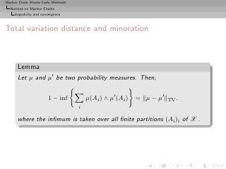
Properties
The resulting sample is not iid but there exist strong convergence
properties:
Theorem (Ergodicity)
The algorithm produces a uniformly ergodic chain if there exists a
constant M such that
f (x) ≤ M g(x) , x ∈ supp f.
In this case,
n
n 1
K (x, ·) − f TV ≤ 1− .
M
[Mengersen & Tweedie, 1996]](https://image.slidesharecdn.com/main-091109121752-phpapp01/85/Monte-Carlo-Statistical-Methods-300-320.jpg?cb=1713217764)


![Markov Chain Monte Carlo Methods
The Metropolis-Hastings Algorithm
A collection of Metropolis-Hastings algorithms
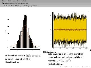
Example (Cauchy by normal)
Given a Cauchy C (0, 1) distribution, consider a normal
go random W
N (0, 1) proposal
The Metropolis–Hastings acceptance ratio is
π(ξ ′ )/ν(ξ ′ ) 1 + (ξ ′ )2
= exp ξ 2 − (ξ ′ )2 /2 .
π(ξ)/ν(ξ)) (1 + ξ 2 )
Poor perfomances: the proposal distribution has lighter tails than
the target Cauchy and convergence to the stationary distribution is
not even geometric!
[Mengersen & Tweedie, 1996]](https://image.slidesharecdn.com/main-091109121752-phpapp01/85/Monte-Carlo-Statistical-Methods-308-320.jpg?cb=1713217764)


![Markov Chain Monte Carlo Methods
The Metropolis-Hastings Algorithm
A collection of Metropolis-Hastings algorithms
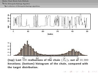
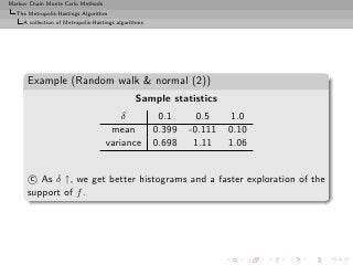
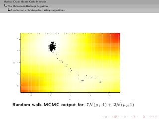
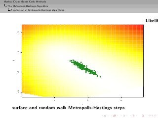
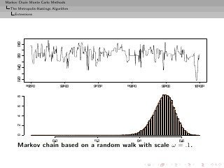
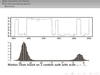
Example (Random walk and normal target)
Generate N (0, 1) based on the uniform proposal [−δ, δ]
forget History!
[Hastings (1970)]
The probability of acceptance is then
2
ρ(x(t) , yt ) = exp{(x(t) − yt )/2} ∧ 1.
2](https://image.slidesharecdn.com/main-091109121752-phpapp01/85/Monte-Carlo-Statistical-Methods-312-320.jpg?cb=1713217764)
![Markov Chain Monte Carlo Methods
The Metropolis-Hastings Algorithm
A collection of Metropolis-Hastings algorithms
400
400
250
0.5
0.5
0.5
300
200
300
0.0
0.0
0.0
150
200
200
-0.5
-0.5
-0.5
100
100
100
-1.0
-1.0
-1.0
50
-1.5
-1.5
-1.5
0
0
0
-1 0 1 2 -2 0 2 -3 -2 -1 0 1 2 3
(a) (b) (c)
Three samples based on U[−δ, δ] with (a) δ = 0.1, (b) δ = 0.5
and (c) δ = 1.0, superimposed with the convergence of the
means (15, 000 simulations).](https://image.slidesharecdn.com/main-091109121752-phpapp01/85/Monte-Carlo-Statistical-Methods-314-320.jpg?cb=1713217764)


![Markov Chain Monte Carlo Methods
The Metropolis-Hastings Algorithm
A collection of Metropolis-Hastings algorithms
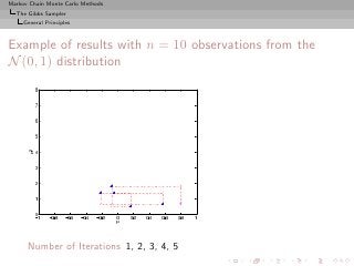
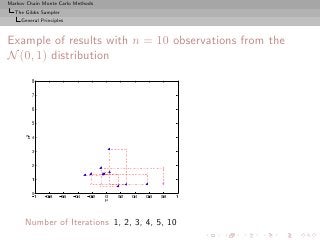
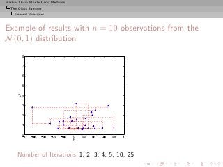
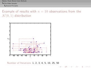
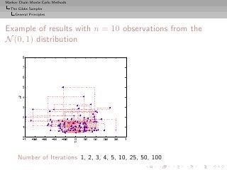
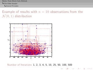
Random walk sampling (50000 iterations)
2
2
1
1
theta
theta
0
0
-1
-1
0.0 0.2 0.4 0.6 0.8 1.0 0.2 0.4 0.6 0.8 1.0 1.2
p tau
1.2
0.0 1.0 2.0
1.0
-1 0 1 2
theta
0.8
0 1 2 3 4 5 6
tau
0.6
0.4
0.0 0.2 0.4 0.6 0.8 1.0
p
0 2 4
0.2
0.0 0.2 0.4 0.6 0.8 1.0 0.2 0.4 0.6 0.8
p tau
General case of a 3 component normal mixture
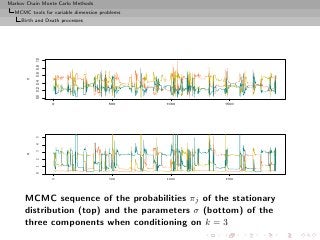
[Celeux & al., 2000]](https://image.slidesharecdn.com/main-091109121752-phpapp01/85/Monte-Carlo-Statistical-Methods-317-320.jpg?cb=1713217764)


![Markov Chain Monte Carlo Methods
The Metropolis-Hastings Algorithm
A collection of Metropolis-Hastings algorithms
Convergence properties
Uniform ergodicity prohibited by random walk structure
At best, geometric ergodicity:
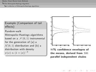
Theorem (Sufficient ergodicity)
For a symmetric density f , log-concave in the tails, and a positive
and symmetric density g, the chain (X (t) ) is geometrically ergodic.
[Mengersen & Tweedie, 1996]
no tail effect](https://image.slidesharecdn.com/main-091109121752-phpapp01/85/Monte-Carlo-Statistical-Methods-323-320.jpg?cb=1713217764)
![Markov Chain Monte Carlo Methods
The Metropolis-Hastings Algorithm
A collection of Metropolis-Hastings algorithms
Example (Cauchy by normal continued)
Again, Cauchy C (0, 1) target and Gaussian random walk proposal,
ξ ′ ∼ N (ξ, σ 2 ), with acceptance probability
1 + ξ2
∧ 1,
1 + (ξ ′ )2
Overall fit of the Cauchy density by the histogram satisfactory, but
poor exploration of the tails: 99% quantile of C (0, 1) equal to 3,
but no simulation exceeds 14 out of 10, 000!
[Roberts & Tweedie, 2004]](https://image.slidesharecdn.com/main-091109121752-phpapp01/85/Monte-Carlo-Statistical-Methods-325-320.jpg?cb=1713217764)
![Markov Chain Monte Carlo Methods
The Metropolis-Hastings Algorithm
A collection of Metropolis-Hastings algorithms
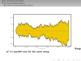
Again, lack of geometric ergodicity!
[Mengersen & Tweedie, 1996]
Slow convergence shown by the non-stable range after 10, 000
iterations.
0.35
0.30
0.25
0.20
Density
0.15
0.10
0.05
0.00
−5 0 5
Histogram of the 10, 000 first steps of a random walk
Metropolis–Hastings algorithm using a N (ξ, 1) proposal](https://image.slidesharecdn.com/main-091109121752-phpapp01/85/Monte-Carlo-Statistical-Methods-326-320.jpg?cb=1713217764)
![Markov Chain Monte Carlo Methods
The Metropolis-Hastings Algorithm
A collection of Metropolis-Hastings algorithms
Further convergence properties
Under assumptions skip detailed convergence
◮ (A1) f is super-exponential, i.e. it is positive with positive
continuous first derivative such that
lim|x|→∞ n(x)′ ∇ log f (x) = −∞ where n(x) := x/|x|.
In words : exponential decay of f in every direction with rate
tending to ∞
◮ (A2) lim sup|x|→∞ n(x)′ m(x) < 0, where
m(x) = ∇f (x)/|∇f (x)|.
In words: non degeneracy of the countour manifold
Cf (y) = {y : f (y) = f (x)}
Q is geometrically ergodic, and
V (x) ∝ f (x)−1/2 verifies the drift condition
[Jarner & Hansen, 2000]](https://image.slidesharecdn.com/main-091109121752-phpapp01/85/Monte-Carlo-Statistical-Methods-328-320.jpg?cb=1713217764)
![Markov Chain Monte Carlo Methods
The Metropolis-Hastings Algorithm
A collection of Metropolis-Hastings algorithms
Further [further] convergence properties
skip hyperdetailed convergence
If P ψ-irreducible and aperiodic, for r = (r(n))n∈N real-valued non
decreasing sequence, such that, for all n, m ∈ N,
r(n + m) ≤ r(n)r(m),
and r(0) = 1, for C a small set, τC = inf{n ≥ 1, Xn ∈ C}, and
h ≥ 1, assume
τC −1
sup Ex r(k)h(Xk ) < ∞,
x∈C k=0](https://image.slidesharecdn.com/main-091109121752-phpapp01/85/Monte-Carlo-Statistical-Methods-329-320.jpg?cb=1713217764)
![Markov Chain Monte Carlo Methods
The Metropolis-Hastings Algorithm
A collection of Metropolis-Hastings algorithms
then,
τC −1
S(f, C, r) := x ∈ X, Ex r(k)h(Xk ) <∞
k=0
is full and absorbing and for x ∈ S(f, C, r),
lim r(n) P n (x, .) − f h = 0.
n→∞
[Tuominen & Tweedie, 1994]](https://image.slidesharecdn.com/main-091109121752-phpapp01/85/Monte-Carlo-Statistical-Methods-330-320.jpg?cb=1713217764)
![Markov Chain Monte Carlo Methods
The Metropolis-Hastings Algorithm
A collection of Metropolis-Hastings algorithms
Comments
◮ [CLT, Rosenthal’s inequality...] h-ergodicity implies CLT
for additive (possibly unbounded) functionals of the chain,
Rosenthal’s inequality and so on...
◮ [Control of the moments of the return-time] The
condition implies (because h ≥ 1) that
τC −1
sup Ex [r0 (τC )] ≤ sup Ex r(k)h(Xk ) < ∞,
x∈C x∈C k=0
where r0 (n) = n r(l) Can be used to derive bounds for
l=0
the coupling time, an essential step to determine computable
bounds, using coupling inequalities
[Roberts & Tweedie, 1998; Fort & Moulines, 2000]](https://image.slidesharecdn.com/main-091109121752-phpapp01/85/Monte-Carlo-Statistical-Methods-331-320.jpg?cb=1713217764)
![Markov Chain Monte Carlo Methods
The Metropolis-Hastings Algorithm
A collection of Metropolis-Hastings algorithms
Alternative conditions
The condition is not really easy to work with...
[Possible alternative conditions]
(a) [Tuominen, Tweedie, 1994] There exists a sequence
(Vn )n∈N , Vn ≥ r(n)h, such that
(i) supC V0 < ∞,
(ii) {V0 = ∞} ⊂ {V1 = ∞} and
(iii) P Vn+1 ≤ Vn − r(n)h + br(n)IC .](https://image.slidesharecdn.com/main-091109121752-phpapp01/85/Monte-Carlo-Statistical-Methods-332-320.jpg?cb=1713217764)
![Markov Chain Monte Carlo Methods
The Metropolis-Hastings Algorithm
A collection of Metropolis-Hastings algorithms
(b) [Fort 2000] ∃V ≥ f ≥ 1 and b < ∞, such that supC V < ∞
and
σC
P V (x) + Ex ∆r(k)f (Xk ) ≤ V (x) + bIC (x)
k=0
where σC is the hitting time on C and
∆r(k) = r(k) − r(k − 1), k ≥ 1 and ∆r(0) = r(0).
τC −1
Result (a) ⇔ (b) ⇔ supx∈C Ex k=0 r(k)f (Xk ) < ∞.](https://image.slidesharecdn.com/main-091109121752-phpapp01/85/Monte-Carlo-Statistical-Methods-333-320.jpg?cb=1713217764)


![Markov Chain Monte Carlo Methods
The Metropolis-Hastings Algorithm
Extensions
MH correction
Accept the new value Yt with probability
2
σ2
exp − Yt − x(t) − (t)
2 ∇ log f (x ) 2σ 2
f (Yt )
· ∧1.
f (x(t) ) σ2
2
exp − x(t) − Yt − 2 ∇ log f (Yt ) 2σ 2
Choice of the scaling factor σ
Should lead to an acceptance rate of 0.574 to achieve optimal
convergence rates (when the components of x are uncorrelated)
[Roberts & Rosenthal, 1998]](https://image.slidesharecdn.com/main-091109121752-phpapp01/85/Monte-Carlo-Statistical-Methods-338-320.jpg?cb=1713217764)

![Markov Chain Monte Carlo Methods
The Metropolis-Hastings Algorithm
Extensions
Case of the independent Metropolis–Hastings algorithm
Choice of g that maximizes the average acceptance rate
f (Y ) g(X)
ρ = E min ,1
f (X) g(Y )
f (Y ) f (X)
= 2P ≥ , X ∼ f, Y ∼ g,
g(Y ) g(X)
Related to the speed of convergence of
T
1
h(X (t) )
T
t=1
to Ef [h(X)] and to the ability of the algorithm to explore any
complexity of f](https://image.slidesharecdn.com/main-091109121752-phpapp01/85/Monte-Carlo-Statistical-Methods-340-320.jpg?cb=1713217764)


![Markov Chain Monte Carlo Methods
The Metropolis-Hastings Algorithm
Extensions
Example (Inverse Gaussian distribution (2))
The analytical optimization (in β) of
θ2
M (β) = (x∗ )−α−1/2 exp (β − θ1 )x∗ −
β β
x∗
β
is impossible
β 0.2 0.5 0.8 0.9 1 1.1 1.2 1.5
ρ(β)
ˆ 0.22 0.41 0.54 0.56 0.60 0.63 0.64 0.71
E[Z] 1.137 1.158 1.164 1.154 1.133 1.148 1.181 1.148
E[1/Z] 1.116 1.108 1.116 1.115 1.120 1.126 1.095 1.115
(θ1 = 1.5, θ2 = 2, and m = 5000).](https://image.slidesharecdn.com/main-091109121752-phpapp01/85/Monte-Carlo-Statistical-Methods-344-320.jpg?cb=1713217764)


![Markov Chain Monte Carlo Methods
The Metropolis-Hastings Algorithm
Extensions
Rule of thumb
In small dimensions, aim at an average acceptance rate of 50%. In
large dimensions, at an average acceptance rate of 25%.
[Gelman,Gilks and Roberts, 1995]](https://image.slidesharecdn.com/main-091109121752-phpapp01/85/Monte-Carlo-Statistical-Methods-348-320.jpg?cb=1713217764)
![Markov Chain Monte Carlo Methods
The Metropolis-Hastings Algorithm
Extensions
Rule of thumb
In small dimensions, aim at an average acceptance rate of 50%. In
large dimensions, at an average acceptance rate of 25%.
[Gelman,Gilks and Roberts, 1995]
This rule is to be taken with a pinch of salt!](https://image.slidesharecdn.com/main-091109121752-phpapp01/85/Monte-Carlo-Statistical-Methods-349-320.jpg?cb=1713217764)


![Markov Chain Monte Carlo Methods
The Gibbs Sampler
Completion
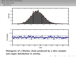
Algorithm (Slice sampler)
Simulate
(t+1)
1. ω1 ∼ U[0,f1 (θ(t) )] ;
...
(t+1)
k. ωk ∼ U[0,fk (θ(t) )] ;
k+1. θ(t+1) ∼ UA(t+1) , with
(t+1)
A(t+1) = {y; fi (y) ≥ ωi , i = 1, . . . , k}.](https://image.slidesharecdn.com/main-091109121752-phpapp01/85/Monte-Carlo-Statistical-Methods-392-320.jpg?cb=1713217764)


![Markov Chain Monte Carlo Methods
The Gibbs Sampler
Convergence
Properties of the Gibbs sampler
Theorem (Convergence)
For
(Y1 , Y2 , · · · , Yp ) ∼ g(y1 , . . . , yp ),
if either
[Positivity condition]
(i) g (i) (y > 0 for every i = 1, · · · , p, implies that
i)
g(y1 , . . . , yp ) > 0, where g (i) denotes the marginal distribution
of Yi , or
(ii) the transition kernel is absolutely continuous with respect to g,
then the chain is irreducible and positive Harris recurrent.](https://image.slidesharecdn.com/main-091109121752-phpapp01/85/Monte-Carlo-Statistical-Methods-404-320.jpg?cb=1713217764)

![Markov Chain Monte Carlo Methods
The Gibbs Sampler
Convergence
Slice sampler
fast on that slice
For convergence, the properties of Xt and of f (Xt ) are identical
Theorem (Uniform ergodicity)
If f is bounded and suppf is bounded, the simple slice sampler is
uniformly ergodic.
[Mira & Tierney, 1997]](https://image.slidesharecdn.com/main-091109121752-phpapp01/85/Monte-Carlo-Statistical-Methods-406-320.jpg?cb=1713217764)
![Markov Chain Monte Carlo Methods
The Gibbs Sampler
Convergence
A small set for a slice sampler
no slice detail
For ǫ⋆ > ǫ⋆ ,
C = {x ∈ X ; ǫ⋆ < f (x) < ǫ⋆ }
is a small set:
ǫ⋆
Pr(x, ·) ≥ µ(·)
ǫ⋆
where ǫ⋆
1 λ(A ∩ L(ǫ))
µ(A) = dǫ
ǫ⋆ 0 λ(L(ǫ))
if L(ǫ) = {x ∈ X ; f (x) > ǫ}‘
[Roberts & Rosenthal, 1998]](https://image.slidesharecdn.com/main-091109121752-phpapp01/85/Monte-Carlo-Statistical-Methods-407-320.jpg?cb=1713217764)
![Markov Chain Monte Carlo Methods
The Gibbs Sampler
Convergence
Slice sampler: drift
Under differentiability and monotonicity conditions, the slice
sampler also verifies a drift condition with V (x) = f (x)−β , is
geometrically ergodic, and there even exist explicit bounds on the
total variation distance
[Roberts & Rosenthal, 1998]](https://image.slidesharecdn.com/main-091109121752-phpapp01/85/Monte-Carlo-Statistical-Methods-408-320.jpg?cb=1713217764)
![Markov Chain Monte Carlo Methods
The Gibbs Sampler
Convergence
Slice sampler: drift
Under differentiability and monotonicity conditions, the slice
sampler also verifies a drift condition with V (x) = f (x)−β , is
geometrically ergodic, and there even exist explicit bounds on the
total variation distance
[Roberts & Rosenthal, 1998]
Example (Exponential Exp(1))
For n > 23,
||K n (x, ·) − f (·)||T V ≤ .054865 (0.985015)n (n − 15.7043)](https://image.slidesharecdn.com/main-091109121752-phpapp01/85/Monte-Carlo-Statistical-Methods-409-320.jpg?cb=1713217764)
![Markov Chain Monte Carlo Methods
The Gibbs Sampler
Convergence
Slice sampler: convergence
no more slice detail
Theorem
For any density such that
∂
ǫ λ ({x ∈ X ; f (x) > ǫ}) is non-increasing
∂ǫ
then
||K 523 (x, ·) − f (·)||T V ≤ .0095
[Roberts & Rosenthal, 1998]](https://image.slidesharecdn.com/main-091109121752-phpapp01/85/Monte-Carlo-Statistical-Methods-410-320.jpg?cb=1713217764)

![Markov Chain Monte Carlo Methods
The Gibbs Sampler
The Hammersley-Clifford theorem
Hammersley-Clifford theorem
An illustration that conditionals determine the joint distribution
Theorem
If the joint density g(y1 , y2 ) have conditional distributions
g1 (y1 |y2 ) and g2 (y2 |y1 ), then
g2 (y2 |y1 )
g(y1 , y2 ) = .
g2 (v|y1 )/g1 (y1 |v) dv
[Hammersley & Clifford, circa 1970]](https://image.slidesharecdn.com/main-091109121752-phpapp01/85/Monte-Carlo-Statistical-Methods-412-320.jpg?cb=1713217764)


![Markov Chain Monte Carlo Methods
The Gibbs Sampler
Hierarchical models
Example (Animal epidemiology (2))
Modified model
Xi ∼ P(λi )
λi ∼ G a(α, βi )
βi ∼ I G (a, b),
The Gibbs sampler corresponds to conditionals
λi ∼ π(λi |x, α, βi ) = G a(xi + α, [1 + 1/βi ]−1 )
βi ∼ π(βi |x, α, a, b, λi ) = I G (α + a, [λi + 1/b]−1 )](https://image.slidesharecdn.com/main-091109121752-phpapp01/85/Monte-Carlo-Statistical-Methods-416-320.jpg?cb=1713217764)


![Markov Chain Monte Carlo Methods
The Gibbs Sampler
Hierarchical models
Conditional decompositions (3)
Moreover, this decomposition works for the posterior moments,
that is, for every function h,
Eπ [h(θ)|x] = Eπ(θ1 |x) [Eπ1 [h(θ)|θ1 , x]] ,
where
Eπ1 [h(θ)|θ1 , x] = h(θ)π(θ|θ1 , x) dθ.
Θ](https://image.slidesharecdn.com/main-091109121752-phpapp01/85/Monte-Carlo-Statistical-Methods-422-320.jpg?cb=1713217764)


![Markov Chain Monte Carlo Methods
The Gibbs Sampler
Hierarchical models
Posterior Gibbs inference
µδ µD µP µD − µP
Probability 1.00 0.9998 0.94 0.985
Confidence [-3.48,-2.17] [0.94,2.50] [-0.17,1.24] [0.14,2.20]
Posterior probabilities of significant effects](https://image.slidesharecdn.com/main-091109121752-phpapp01/85/Monte-Carlo-Statistical-Methods-426-320.jpg?cb=1713217764)


![Markov Chain Monte Carlo Methods
The Gibbs Sampler
Data Augmentation
Rao-Blackwellization (2)
Then
◦ Both estimators converge to E[h(Y1 )]
◦ Both are unbiased,](https://image.slidesharecdn.com/main-091109121752-phpapp01/85/Monte-Carlo-Statistical-Methods-436-320.jpg?cb=1713217764)
![Markov Chain Monte Carlo Methods
The Gibbs Sampler
Data Augmentation
Rao-Blackwellization (2)
Then
◦ Both estimators converge to E[h(Y1 )]
◦ Both are unbiased,
◦ and
(t)
var E h(Y1 )|Y2 , . . . , Yp(t) ≤ var(h(Y1 )),
so δrb is uniformly better (for Data Augmentation)](https://image.slidesharecdn.com/main-091109121752-phpapp01/85/Monte-Carlo-Statistical-Methods-437-320.jpg?cb=1713217764)
![Markov Chain Monte Carlo Methods
The Gibbs Sampler
Data Augmentation
Examples of Rao-Blackwellization
Example
Bivariate normal Gibbs sampler
X | y ∼ N (ρy, 1 − ρ2 )
Y | x ∼ N (ρx, 1 − ρ2 ).
Then
T T T
1 1 1
δ0 = X (i) and δ1 = E[X (i) |Y (i) ] = ̺Y (i) ,
T T T
i=1 i=1 i=1
2 2 1
estimate E[X] and σδ0 /σδ1 = ρ2
> 1.](https://image.slidesharecdn.com/main-091109121752-phpapp01/85/Monte-Carlo-Statistical-Methods-438-320.jpg?cb=1713217764)
![Markov Chain Monte Carlo Methods
The Gibbs Sampler
Data Augmentation
Examples of Rao-Blackwellization (2)
Example (Poisson-Gamma Gibbs cont’d)
Na¨ estimate
ıve
T
1
δ0 = λ(t)
T
t=1
and Rao-Blackwellized version
T
1 (i) (i) (i)
δπ = E[λ(t) |x1 , x2 , . . . , x5 , y1 , y2 , . . . , y13 ]
T
t=1
T 13
1 (t)
= 313 + yi ,
360T
t=1 i=1
back to graph](https://image.slidesharecdn.com/main-091109121752-phpapp01/85/Monte-Carlo-Statistical-Methods-439-320.jpg?cb=1713217764)


![Markov Chain Monte Carlo Methods
MCMC tools for variable dimension problems
Introduction
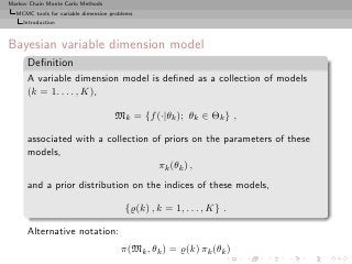
A new brand of problems
There exist setups where
One of the things we do not know is the number
of things we do not know
[Peter Green]](https://image.slidesharecdn.com/main-091109121752-phpapp01/85/Monte-Carlo-Statistical-Methods-456-320.jpg?cb=1713217764)


![Markov Chain Monte Carlo Methods
MCMC tools for variable dimension problems
Introduction
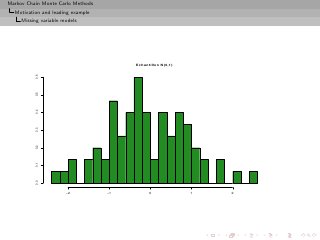
Example (Mixture again, yes!)
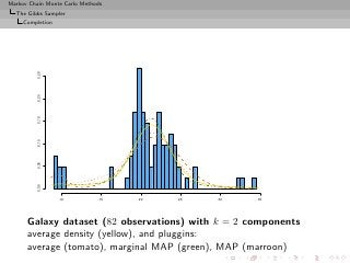
Benchmark dataset: Speed of galaxies
[Roeder, 1990; Richardson & Green, 1997]
2.0
1.5
1.0
0.5
0.0
1.0 1.5 2.0 2.5 3.0 3.5
speeds](https://image.slidesharecdn.com/main-091109121752-phpapp01/85/Monte-Carlo-Statistical-Methods-459-320.jpg?cb=1713217764)

![Markov Chain Monte Carlo Methods
MCMC tools for variable dimension problems
Introduction
Bayesian solution
Formally over:
1. Compute
pi fi (x|θi )πi (θi )dθi
Θi
p(Mi |x) =
pj fj (x|θj )πj (θj )dθj
j Θj
2. Take largest p(Mi |x) to determine model, or use
pj fj (x|θj )πj (θj )dθj
j Θj
as predictive
[Different decision theoretic perspectives]](https://image.slidesharecdn.com/main-091109121752-phpapp01/85/Monte-Carlo-Statistical-Methods-462-320.jpg?cb=1713217764)
![Markov Chain Monte Carlo Methods
MCMC tools for variable dimension problems
Introduction
Difficulties
Not at
◮ (formal) inference level [see above]
◮ parameter space representation
Θ= Θk ,
k
[even if there are parameters common to several models]](https://image.slidesharecdn.com/main-091109121752-phpapp01/85/Monte-Carlo-Statistical-Methods-463-320.jpg?cb=1713217764)
![Markov Chain Monte Carlo Methods
MCMC tools for variable dimension problems
Introduction
Difficulties
Not at
◮ (formal) inference level [see above]
◮ parameter space representation
Θ= Θk ,
k
[even if there are parameters common to several models]
Rather at
◮ (practical) inference level:
model separation, interpretation, overfitting, prior modelling,
prior coherence
◮ computational level:
infinity of models, moves between models, predictive
computation](https://image.slidesharecdn.com/main-091109121752-phpapp01/85/Monte-Carlo-Statistical-Methods-464-320.jpg?cb=1713217764)
![Markov Chain Monte Carlo Methods
MCMC tools for variable dimension problems
Green’s method
Green’s resolution
Setting up a proper measure–theoretic framework for designing
moves between models Mk
[Green, 1995]](https://image.slidesharecdn.com/main-091109121752-phpapp01/85/Monte-Carlo-Statistical-Methods-465-320.jpg?cb=1713217764)
![Markov Chain Monte Carlo Methods
MCMC tools for variable dimension problems
Green’s method
Green’s resolution
Setting up a proper measure–theoretic framework for designing
moves between models Mk
[Green, 1995]
Create a reversible kernel K on H = k {k} × Θk such that
K(x, dy)π(x)dx = K(y, dx)π(y)dy
A B B A
for the invariant density π [x is of the form (k, θ(k) )]](https://image.slidesharecdn.com/main-091109121752-phpapp01/85/Monte-Carlo-Statistical-Methods-466-320.jpg?cb=1713217764)


![Markov Chain Monte Carlo Methods
MCMC tools for variable dimension problems
Green’s method
Saturation
[Brooks, Giudici, Roberts, 2003]
Consider series of models Mi (i = 1, . . . , k) such that
max dim(Mi ) = nmax < ∞
i
Parameter of model Mi then completed with an auxiliary variable
Ui such that
dim(θi , ui ) = nmax and Ui ∼ qi (ui )
Posit the following joint distribution for [augmented] model Mi
π(Mi , θi ) qi (ui )](https://image.slidesharecdn.com/main-091109121752-phpapp01/85/Monte-Carlo-Statistical-Methods-478-320.jpg?cb=1713217764)


![Markov Chain Monte Carlo Methods
MCMC tools for variable dimension problems
Green’s method
Example (Mixture of normal distributions)
k
2
Mk : pjk N (µjk , σjk )
j=1
[Richardson & Green, 1997]
Moves:](https://image.slidesharecdn.com/main-091109121752-phpapp01/85/Monte-Carlo-Statistical-Methods-481-320.jpg?cb=1713217764)
![Markov Chain Monte Carlo Methods
MCMC tools for variable dimension problems
Green’s method
Example (Mixture of normal distributions)
k
2
Mk : pjk N (µjk , σjk )
j=1
[Richardson & Green, 1997]
Moves:
(i) Split
pjk = pj(k+1) + p(j+1)(k+1)
pjk µjk = pj(k+1) µj(k+1) + p(j+1)(k+1) µ(j+1)(k+1)
2 2 2
pjk σjk = pj(k+1) σj(k+1) + p(j+1)(k+1) σ(j+1)(k+1)
(ii) Merge (reverse)](https://image.slidesharecdn.com/main-091109121752-phpapp01/85/Monte-Carlo-Statistical-Methods-482-320.jpg?cb=1713217764)


![Markov Chain Monte Carlo Methods
MCMC tools for variable dimension problems
Green’s method
Example (Hidden Markov model (2))
Move to split component j⋆ into j1 and j2 :
ωij1 = ωij⋆ εi , ωij2 = ωij⋆ (1 − εi ), εi ∼ U(0, 1);
ωj1 j = ωj⋆ j ξj , ωj2 j = ωj⋆ j /ξj , ξj ∼ log N (0, 1);
similar ideas give ωj1 j2 etc.;
µj1 = µj⋆ − 3σj⋆ εµ , µj2 = µj⋆ + 3σj⋆ εµ , εµ ∼ N (0, 1);
2 2 2 2
σj1 = σj∗ ξσ , σj2 = σj∗ /ξσ , ξσ ∼ log N (0, 1).
[Robert al., 2000]](https://image.slidesharecdn.com/main-091109121752-phpapp01/85/Monte-Carlo-Statistical-Methods-487-320.jpg?cb=1713217764)

![Markov Chain Monte Carlo Methods
MCMC tools for variable dimension problems
Green’s method
Example (Autoregressive model)
move to birth
Typical setting for model choice: determine order p of AR(p)
model
Consider the (less standard) representation
p
(1 − λi B) Xt = ǫt , ǫt ∼ N (0, σ 2 )
i=1
where the λi ’s are within the unit circle if complex and within
[−1, 1] if real.
[Huerta and West, 1998]](https://image.slidesharecdn.com/main-091109121752-phpapp01/85/Monte-Carlo-Statistical-Methods-490-320.jpg?cb=1713217764)
![Markov Chain Monte Carlo Methods
MCMC tools for variable dimension problems
Green’s method
AR(p) reversible jump algorithm
Example (Autoregressive (2))
Uniform priors for the real and complex roots λj ,
1 1 1
I I
⌊k/2⌋ + 1 2 |λi |1 π |λi |1
λi ∈R λi ∈R
and (purely birth-and-death) proposals based on these priors
◮ k → k+1 [Creation of real root]
◮ k → k+2 [Creation of complex root]
◮ k → k-1 [Deletion of real root]
◮ k → k-2 [Deletion of complex root]](https://image.slidesharecdn.com/main-091109121752-phpapp01/85/Monte-Carlo-Statistical-Methods-491-320.jpg?cb=1713217764)
![Markov Chain Monte Carlo Methods
MCMC tools for variable dimension problems
Birth and Death processes
Birth and Death processes
instant death!
Use of an alternative methodology based on a Birth–-Death
(point) process
[Preston, 1976; Ripley, 1977; Geyer Møller, 1994; Stevens, 1999]](https://image.slidesharecdn.com/main-091109121752-phpapp01/85/Monte-Carlo-Statistical-Methods-492-320.jpg?cb=1713217764)
![Markov Chain Monte Carlo Methods
MCMC tools for variable dimension problems
Birth and Death processes
Birth and Death processes
instant death!
Use of an alternative methodology based on a Birth–-Death
(point) process
[Preston, 1976; Ripley, 1977; Geyer Møller, 1994; Stevens, 1999]
Idea: Create a Markov chain in continuous time, i.e. a Markov
jump process, moving between models Mk , by births (to increase
the dimension), deaths (to decrease the dimension), and other
moves.](https://image.slidesharecdn.com/main-091109121752-phpapp01/85/Monte-Carlo-Statistical-Methods-493-320.jpg?cb=1713217764)


![Markov Chain Monte Carlo Methods
MCMC tools for variable dimension problems
Birth and Death processes
Stephen’s original algorithm
Algorithm (Mixture Birth Death)
For v = 0, 1, · · · , V
t←v
Run till t v + 1
L(Φ|Φj ) λ0
1. Compute δj (Φ) =
L(Φ) λ1
k
2. δ(Φ) ← δj (Φj ), ξ ← λ0 + δ(Φ), u ∼ U([0, 1])
j=1
3. t ← t − u log(u)](https://image.slidesharecdn.com/main-091109121752-phpapp01/85/Monte-Carlo-Statistical-Methods-499-320.jpg?cb=1713217764)


![Markov Chain Monte Carlo Methods
MCMC tools for variable dimension problems
Birth and Death processes
Example (HMM models (cont’d))
Implementation of the split-and-combine rule of Richardson and
Green (1997) in continuous time
Move to split component j∗ into j1 and j2 :
ωij1 = ωij∗ ǫi , ωij2 = ωij∗ (1 − ǫi ), ǫi ∼ U(0, 1);
ωj1 j = ωj∗ j ξj , ωj2 j = ωj∗ j /ξj , ξj ∼ log N (0, 1);
similar ideas give ωj1 j2 etc.;
µj1 = µj∗ − 3σj∗ ǫµ , µj2 = µj∗ + 3σj∗ ǫµ , ǫµ ∼ N (0, 1);
2 2 2 2
σj1 = σj∗ ξσ , σj2 = σj∗ /ξσ , ξσ ∼ log N (0, 1).
[Capp´ al, 2001]
e](https://image.slidesharecdn.com/main-091109121752-phpapp01/85/Monte-Carlo-Statistical-Methods-503-320.jpg?cb=1713217764)

![Markov Chain Monte Carlo Methods
MCMC tools for variable dimension problems
Birth and Death processes
Number of states
5
Relative Frequency
0.6
number of states
4
0.4
3
0.2
2
0.0
1
2 4 6 8 10 0 500 1000 1500 2000 2500
temp[, 1] instants
Log likelihood values
−200
0.030
Relative Frequency
−1400 −1000 −600
0.020
log−likelihood
0.010
0.000
−1400 −1200 −1000 −800 −600 −400 −200 0 500 1000 1500 2000 2500
temp[, 2] instants
Number of moves
30
0.00 0.05 0.10 0.15
Relative Frequency
Number of moves
20
5 10
5 10 15 20 25 30 0 500 1000 1500 2000 2500
temp[, 3] instants
MCMC output on k (histogram and rawplot), corresponding
loglikelihood values (histogram and rawplot), and number of
moves (histogram and rawplot)](https://image.slidesharecdn.com/main-091109121752-phpapp01/85/Monte-Carlo-Statistical-Methods-505-320.jpg?cb=1713217764)


![Markov Chain Monte Carlo Methods
Sequential importance sampling
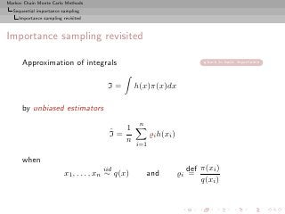
Importance sampling revisited
Markov extension
For densities f and g, and importance weight
ω(x) = f (x)/g(x) ,
for any kernel K(x, x′ ) with stationary distribution f ,
ω(x) K(x, x′ ) g(x)dx = f (x′ ) .
[McEachern, Clyde, and Liu, 1999]](https://image.slidesharecdn.com/main-091109121752-phpapp01/85/Monte-Carlo-Statistical-Methods-519-320.jpg?cb=1713217764)
![Markov Chain Monte Carlo Methods
Sequential importance sampling
Importance sampling revisited
Markov extension
For densities f and g, and importance weight
ω(x) = f (x)/g(x) ,
for any kernel K(x, x′ ) with stationary distribution f ,
ω(x) K(x, x′ ) g(x)dx = f (x′ ) .
[McEachern, Clyde, and Liu, 1999]
Consequence: An importance sample transformed by MCMC
transitions keeps its weights
Unbiasedness preservation:
E ω(X)h(X ′ ) = ω(x) h(x′ ) K(x, x′ ) g(x) dx dx′
= Ef [h(X)]](https://image.slidesharecdn.com/main-091109121752-phpapp01/85/Monte-Carlo-Statistical-Methods-520-320.jpg?cb=1713217764)


![Markov Chain Monte Carlo Methods
Sequential importance sampling
Dynamic extensions
Dynamic importance sampling
Idea
It is possible to generalise importance sampling using random
weights ωt such that
E[ωt |xt ] = π(xt )/g(xt )](https://image.slidesharecdn.com/main-091109121752-phpapp01/85/Monte-Carlo-Statistical-Methods-525-320.jpg?cb=1713217764)
![Markov Chain Monte Carlo Methods
Sequential importance sampling
Dynamic extensions
(a) Self-regenerative chains
[Sahu Zhigljavsky, 1998; Gasemyr, 2002]
Proposal
Y ∼ p(y) ∝ p(y)
˜
and target distribution π(y) ∝ π (y)
˜
Ratios
ω(x) = π(x)/p(x) and ω (x) = π (x)/˜(x)
˜ ˜ p
Unknown Known
Acceptance function
1
α(x) = κ0
1 + κ˜ (x)
ω](https://image.slidesharecdn.com/main-091109121752-phpapp01/85/Monte-Carlo-Statistical-Methods-526-320.jpg?cb=1713217764)

![Markov Chain Monte Carlo Methods
Sequential importance sampling
Dynamic extensions
Plusses
◮ Valid for any choice of κ [κ small = large variance and κ large
= slow convergence]
◮ Only depends on current value [Difference with Metropolis]
◮ Random integer weight W [Similarity with Metropolis]
◮ Saves on the rejections: always accept [Difference with
Metropolis]
◮ Introduces geometric noise compared with importance
sampling
2 2 2
σSZ = 2 σIS + (1/κ)σπ
◮ Can be used with a sequence of proposals pk and constants
κk [Adaptativity]](https://image.slidesharecdn.com/main-091109121752-phpapp01/85/Monte-Carlo-Statistical-Methods-528-320.jpg?cb=1713217764)
![Markov Chain Monte Carlo Methods
Sequential importance sampling
Dynamic extensions
A generalisation
[G˚semyr, 2002]
a
Proposal density p(y) and probability q(y) of accepting a jump.](https://image.slidesharecdn.com/main-091109121752-phpapp01/85/Monte-Carlo-Statistical-Methods-529-320.jpg?cb=1713217764)
![Markov Chain Monte Carlo Methods
Sequential importance sampling
Dynamic extensions
A generalisation
[G˚semyr, 2002]
a
Proposal density p(y) and probability q(y) of accepting a jump.
Algorithm (G˚semyr’s dynamic weights)
a
Generate a sequence of random weights Wn by
1. Generate Yn ∼ p(y)
2. Generate Vn ∼ B(q(yn ))
3. Generate Sn ∼ Geo(α(yn ))
4. Take Wn = Vn Sn](https://image.slidesharecdn.com/main-091109121752-phpapp01/85/Monte-Carlo-Statistical-Methods-530-320.jpg?cb=1713217764)


![Markov Chain Monte Carlo Methods
Sequential importance sampling
Dynamic extensions
Ergodicity for G˚semyr’s scheme
a
Necessary and sufficient condition
π is stationary for (Xt ) iff
α(y) = q(y)/(κπ(y)/p(y)) = q(y)/(κw(y))
for some constant κ.
Implies that
E[W n |Y n = y] = κw(y) .
[Average importance sampling]
Special case: α(y) = 1/(1 + κw(y)) of Sahu and Zhigljavski (2001)](https://image.slidesharecdn.com/main-091109121752-phpapp01/85/Monte-Carlo-Statistical-Methods-533-320.jpg?cb=1713217764)

![Markov Chain Monte Carlo Methods
Sequential importance sampling
Dynamic extensions
(b) Dynamic weighting
[Wong Liang, 1997; Liu, Liang Wong, 2001; Liang, 2002]
direct to PMC
Generalisation of the above: simultaneous generation of points
and weights, (θt , ωt ), under the constraint
E[ωt |θt ] ∝ π(θt ) (5)
Same use as importance sampling weights](https://image.slidesharecdn.com/main-091109121752-phpapp01/85/Monte-Carlo-Statistical-Methods-535-320.jpg?cb=1713217764)

![Markov Chain Monte Carlo Methods
Sequential importance sampling
Dynamic extensions
Preservation of the equilibrium equation
If g− and g+ denote the distributions of the augmented variable
(X, W ) before the step and after the step, respectively, then
∞
ω ′ g+ (x′ , ω ′ ) dω ′ =
0
̺(ω, x, x′ )
(1 + δ) [̺(ω, x, x′ ) + θ] g− (x, ω) K(x, x′ ) dx dω
̺(ω, x, x′ ) + θ
ω(̺(ω, x′ , z) + θ) θ
+ (1 + δ) g− (x′ , ω) K(x, z) ′ , z) + θ
dz dω
θ ̺(ω, x
π(x′ )K(x′ , x)
= (1 + δ) ω g− (x, ω) dx dω
π(x)
+ ω g− (x′ , ω) K(x′ , z) dz dω
= (1 + δ) π(x′ ) c0 K(x′ , x) dx + c0 π(x′ )
= 2(1 + δ)c0 π(x′ ) ,](https://image.slidesharecdn.com/main-091109121752-phpapp01/85/Monte-Carlo-Statistical-Methods-537-320.jpg?cb=1713217764)
![Markov Chain Monte Carlo Methods
Sequential importance sampling
Dynamic extensions
Special case: R-move
[Liang, 2002]
δ = 0 and θ ≡ 1, and thus
(y, ̺ + 1) if u ̺/(̺ + 1)
(x′ , ω ′ ) =
(x, ω(̺ + 1)) otherwise,
[Importance sampling]](https://image.slidesharecdn.com/main-091109121752-phpapp01/85/Monte-Carlo-Statistical-Methods-538-320.jpg?cb=1713217764)
![Markov Chain Monte Carlo Methods
Sequential importance sampling
Dynamic extensions
Special case: W -move
θ ≡ 0, thus a = 1 and
(x′ , ω ′ ) = (y, ̺) .
Q-move
[Liu al, 2001]
(y, θ ∨ ̺) if u 1 ∧ ̺/θ ,
(x′ , ω ′ ) =
(x, aω) otherwise,
with a ≥ 1 either a constant or an independent random variable.](https://image.slidesharecdn.com/main-091109121752-phpapp01/85/Monte-Carlo-Statistical-Methods-539-320.jpg?cb=1713217764)


![Markov Chain Monte Carlo Methods
Sequential importance sampling
Dynamic extensions
Notes (2)
◮ Geometric structure of the weights
ωt
Pr(Rt = 0) = .
ωt+1
and
ωt r(xt , yt )
Pr(Rt = 0) = , θ 0,
ωt r(xt , yt ) + θ
for the R scheme
◮ Number of steps T before an acceptance (a jump) such that
Pr (T ≥ t) = P (R1 = 0, . . . , Rt−1 = 0)
t−1
ωj
= E ∝ E[1/ωt ] .
ωj+1
j=0](https://image.slidesharecdn.com/main-091109121752-phpapp01/85/Monte-Carlo-Statistical-Methods-542-320.jpg?cb=1713217764)

![Markov Chain Monte Carlo Methods
Sequential importance sampling
Dynamic extensions
Alternative scheme (2)
Then
Pr (T = t) = P (R1 = 0, . . . , Rt−1 = 0, Rt = 1)
t−1
ωj ωt−1 r(x0 , Yt )
= E αj (1 − αt )
ωj+1 ωt
j=0
which is equal to
αt−1 (1 − α)E[ωo r(x, Yt )/ωt ]
when αj constant and deterministic.](https://image.slidesharecdn.com/main-091109121752-phpapp01/85/Monte-Carlo-Statistical-Methods-544-320.jpg?cb=1713217764)


![Markov Chain Monte Carlo Methods
Sequential importance sampling
Population Monte Carlo
Sequential variance decomposition
Furthermore,
n
ˆ 1 (t) (t)
var It = 2 var ̺i h(xi ) ,
n
i=1
(t) (t)
if var ̺i exists, because the xi ’s are conditionally uncorrelated
Note
(t)
This decomposition is still valid for correlated [in i] xi ’s when
(t)
incorporating weights ̺i](https://image.slidesharecdn.com/main-091109121752-phpapp01/85/Monte-Carlo-Statistical-Methods-549-320.jpg?cb=1713217764)

![Markov Chain Monte Carlo Methods
Sequential importance sampling
Population Monte Carlo
Special case of the product proposal
If
n
(t) (t−1) (t)
qt (x |x )= qit (xi |x(t−1) )
i=1
[Independent proposals]
then
n
ˆ 1 (t) (t)
var It = 2 var ̺i h(xi ) ,
n
i=1](https://image.slidesharecdn.com/main-091109121752-phpapp01/85/Monte-Carlo-Statistical-Methods-551-320.jpg?cb=1713217764)
![Markov Chain Monte Carlo Methods
Sequential importance sampling
Population Monte Carlo
Validation
skip validation
(t) (t) (t) (t)
E ̺i h(Xi ) ̺j h(Xj )
π(xi ) π(xj )
= h(xi ) (t−1) ) q (x |x(t−1) )
h(xj )
qit (xi |x jt j
qit (xi |x(t−1) ) qjt (xj |x(t−1) ) dxi dxj g(x(t−1) )dx(t−1)
= Eπ [h(X)]2
whatever the distribution g on x(t−1)](https://image.slidesharecdn.com/main-091109121752-phpapp01/85/Monte-Carlo-Statistical-Methods-552-320.jpg?cb=1713217764)


![Markov Chain Monte Carlo Methods
Sequential importance sampling
Population Monte Carlo
Sampling importance resampling
Importance sampling from g can also produce samples from the
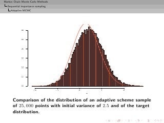
target π
[Rubin, 1987]](https://image.slidesharecdn.com/main-091109121752-phpapp01/85/Monte-Carlo-Statistical-Methods-555-320.jpg?cb=1713217764)
![Markov Chain Monte Carlo Methods
Sequential importance sampling
Population Monte Carlo
Sampling importance resampling
Importance sampling from g can also produce samples from the
target π
[Rubin, 1987]
Theorem (Bootstraped importance sampling)
If a sample (x⋆ )1≤i≤m is derived from the weighted sample
i
(xi , ̺i )1≤i≤n by multinomial sampling with weights ̺i , then
x⋆ ∼ π(x)
i](https://image.slidesharecdn.com/main-091109121752-phpapp01/85/Monte-Carlo-Statistical-Methods-556-320.jpg?cb=1713217764)
![Markov Chain Monte Carlo Methods
Sequential importance sampling
Population Monte Carlo
Sampling importance resampling
Importance sampling from g can also produce samples from the
target π
[Rubin, 1987]
Theorem (Bootstraped importance sampling)
If a sample (x⋆ )1≤i≤m is derived from the weighted sample
i
(xi , ̺i )1≤i≤n by multinomial sampling with weights ̺i , then
x⋆ ∼ π(x)
i
Note
Obviously, the x⋆ ’s are not iid
i](https://image.slidesharecdn.com/main-091109121752-phpapp01/85/Monte-Carlo-Statistical-Methods-557-320.jpg?cb=1713217764)
![Markov Chain Monte Carlo Methods
Sequential importance sampling
Population Monte Carlo
Iterated sampling importance resampling
This principle can be extended to iterated importance sampling:
After each iteration, resampling produces a sample from π
[Again, not iid!]](https://image.slidesharecdn.com/main-091109121752-phpapp01/85/Monte-Carlo-Statistical-Methods-558-320.jpg?cb=1713217764)
![Markov Chain Monte Carlo Methods
Sequential importance sampling
Population Monte Carlo
Iterated sampling importance resampling
This principle can be extended to iterated importance sampling:
After each iteration, resampling produces a sample from π
[Again, not iid!]
Incentive
Use previous sample(s) to learn about π and q](https://image.slidesharecdn.com/main-091109121752-phpapp01/85/Monte-Carlo-Statistical-Methods-559-320.jpg?cb=1713217764)


![Markov Chain Monte Carlo Methods
Sequential importance sampling
Population Monte Carlo
Illustration
Example (A toy example)
Take the target
1/4N (−1, 0.3)(x) + 1/4N (0, 1)(x) + 1/2N (3, 2)(x)
and use 3 proposals: N (−1, 0.3), N (0, 1) and N (3, 2)
[Surprise!!!]](https://image.slidesharecdn.com/main-091109121752-phpapp01/85/Monte-Carlo-Statistical-Methods-577-320.jpg?cb=1713217764)
![Markov Chain Monte Carlo Methods
Sequential importance sampling
Population Monte Carlo
Illustration
Example (A toy example)
Take the target
1/4N (−1, 0.3)(x) + 1/4N (0, 1)(x) + 1/2N (3, 2)(x)
and use 3 proposals: N (−1, 0.3), N (0, 1) and N (3, 2)
[Surprise!!!]
Then
1 0.0500000 0.05000000 0.9000000
2 0.2605712 0.09970292 0.6397259
6 0.2740816 0.19160178 0.5343166
10 0.2989651 0.19200904 0.5090259
16 0.2651511 0.24129039 0.4935585
Weight evolution](https://image.slidesharecdn.com/main-091109121752-phpapp01/85/Monte-Carlo-Statistical-Methods-578-320.jpg?cb=1713217764)
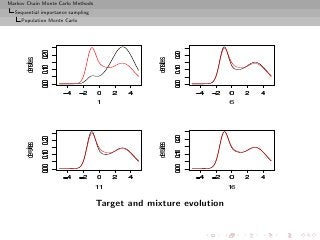


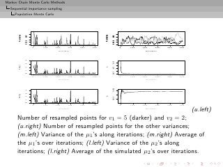


The document discusses Markov Chain Monte Carlo (MCMC) methods, detailing their motivation, applications, and key algorithms such as Metropolis-Hastings and Gibbs sampling. It emphasizes the challenges of latent variable models and the benefits of Bayesian methods in resolving issues like missing data. The document also highlights complications arising from multimodal likelihood functions and the potential limitations of conjugate priors in Bayesian inference.


