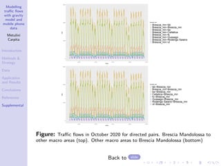
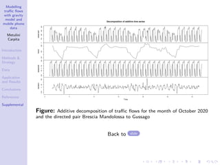
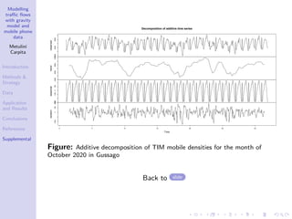
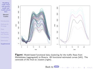
The document discusses a traffic flow modeling project utilizing a gravity model and mobile phone data in the urbanized Mandolossa area of Brescia, Italy, aiming to predict traffic during flood episodes. It outlines the methodology, including data collection and analysis strategies, as well as prior research contributions. Preliminary results indicate promising prediction capabilities and highlight the significance of mobile phone densities and time effects on traffic flows.

1. Modelling
traffic flows
with gravity
model and
mobile phone
data
Metulini
Carpita
Introduction
Methods &
Strategy
Data
Application
and Results
Conclusions
References
Supplemental
Modelling traffic flows with gravity models and
mobile phone large data
Rodolfo Metulini1, Maurizio Carpita2
1. Department of Economics and Statistics - University of Salerno
2. Data Methods and Systems Statistical Laboratory - Department of
Economics and Management, University of Brescia
ODS21 - International Conference on Optimization and Decision
Sciences
September 17th
, 2021

2. Modelling
traffic flows
with gravity
model and
mobile phone
data
Metulini
Carpita
Introduction
Methods &
Strategy
Data
Application
and Results
Conclusions
References
Supplemental
Introduction
• The analysis of origin-destination (O-D) traffic flows is useful in
many contexts of application and they are commonly studied through
the Gravity Model (at least, in economic and statistical disciplines).
• We use a (panel) gravity model to analyse the dynamic of such flows
over the time in the strongly urbanized and flood-prone area of the
Mandolossa (western outskirts of Brescia),
• with the final aim of predict the traffic flow during flood episodes
• Smart cities
• Emergency management plans
• Warning systems

3. Modelling
traffic flows
with gravity
model and
mobile phone
data
Metulini
Carpita
Introduction
Methods &
Strategy
Data
Application
and Results
Conclusions
References
Supplemental
The project
• Ongoing project (’till
06/2022):
MoSoRe@UniBS project:
Project of Lombardy Region, Italy
(Infrastrutture e servizi per la
Mobilità Sostenibile e Resiliente) -
CallHub ID 1180965, bit.ly/2Xh2Nfr
Collaboration with prof. Roberto
Ranzi and the Department of Civil,
Environmental, Architectural
Engineering and Mathematics,
UNIBS
• Scientific output:
1 Metulini, R., Carpita, M., A Spatio-Temporal Indicator for City Users based on Mobile
Phone Signals and Administrative Data - Social Indicator Research, 156, 761–781 (2021).
https://doi.org/10.1007/s11205-020-02355-2
2 Balistrocchi, M., Metulini, R., Carpita, M., and Ranzi, R.: Dynamic maps of people exposure
to floods based on mobile phone data. Natural Hazards and Earth System Sciences, 20,
3485–3500, https://doi.org/10.5194/nhess-20-3485-2020, 2020.

4. Modelling
traffic flows
with gravity
model and
mobile phone
data
Metulini
Carpita
Introduction
Methods &
Strategy
Data
Application
and Results
Conclusions
References
Supplemental
The gravity model
• Tinbergen (1962) firstly applied the concept of Newton’s law to
international trade flows (macro-level)
• The volume of trade between two countries is proportional to
the product of their gross domestic products (GDP) and a
distance deterrence function, called trade resistance
• The popularity of Tinbergen’s log-linear specification is due to its
good modelling performance, and to the strong theoretical
foundations (Anderson, 1979; Anderson & VanWincoop, 2003).
• Gravity model equation has been translated to micro-level flows data
(see, e.g., Barbosa et al., 2018) by substituting (e.g.):
• trade flows with the total number of flows from two regions,
• a measure of dimension of the region of origin and of the region
of destination (such as their population) in place of GDP,
• the geographical (or network) distance among the two regions
in place of trade resistance terms (which includes trade costs).

5. Modelling
traffic flows
with gravity
model and
mobile phone
data
Metulini
Carpita
Introduction
Methods &
Strategy
Data
Application
and Results
Conclusions
References
Supplemental
Gravity model - applied issues
• The classical gravity model reads as:
Fij = G
Mi Mj
Dγ
ij
(1)
where Fij is the flow from origin i to destination j, Mi and Mj are the
masses, Dij is the distance and G and γ are positive constants.
• Introducing the panel dimension and linearising the model using the
logarithmic transformation of (1), the equation assumes the form of a
multiple linear regression with random errors ijt (LeSage Pace,
2009), assuming populations Pi and Pj as masses:
log(Fijt) = α + β1 · log(Pi ) + β2 · log(Pj ) − γ · log(Dij ) + ijt (2)

6. Modelling
traffic flows
with gravity
model and
mobile phone
data
Metulini
Carpita
Introduction
Methods
Strategy
Data
Application
and Results
Conclusions
References
Supplemental
Gravity model - strategy
• Thanks to the availability of a time series of data, we use a most
accurate set of explanatory variables, in order to better account for
the dynamic over the time of the flows:
1 We employ a time-varying mass variable represented by
the density of TIM users1
.
• Densities are estimated from mobile phone data using the
method proposed by Metulini Carpita (2021) and
adopted by Balistrocchi et al. (2020) to derive crowding
maps for flood exposure.
2 A proper set of pure time effects is considered.
• Model (2) can be extended introducing mobile phone densities (MPit
and MPjt), a vector of time effects (TEt) and internal flows (IFij ),
with parameters α, β1, β2, γ, δ1, δ2, ω and λ:
log(Fijt) = α + β1 · log(Pi ) + β2 · log(Pj ) − γ · log(Dij ) + δ1 · log(MPit) +
δ2 · log(MPjt) + ω · IFij + λT
TEt + vijt (3)
1
Average number of mobile phones simultaneously connected to the SIM
network in that area in that time interval, Erlang measure, Carpita Simonetto,
2014)

7. Modelling
traffic flows
with gravity
model and
mobile phone
data
Metulini
Carpita
Introduction
Methods
Strategy
Data
Application
and Results
Conclusions
References
Supplemental
Gravity model - estimation method
• Log-linear specification along with Ordinary Least Squares (OLS) can
be inappropriate, particularly when many zero flows are present.
• Log-linear model with OLS on a truncated sample (dropping zero
flows) can generate biased estimates (Helpman, 2008).
• Santos Silva Tenreyro (2006) shown that log-linearisation leads to
inconsistent estimates in the presence of heteroscedasticity in flows
levels and propose a Poisson specification along with the Poisson
Pseudo Maximum Likelihood (PPML). PPML also better accounts
for zero flows.
• All in all, when just interested on pairs of areas with positive flows, as
in our explorative case study, it is possible to rely on OLS without
particular losses in estimation efficiency.

8. Modelling
traffic flows
with gravity
model and
mobile phone
data
Metulini
Carpita
Introduction
Methods
Strategy
Data
Application
and Results
Conclusions
References
Supplemental
Flow data
• Flow data provided by Olivetti and Fasternet and used by DMS
StatLab.
• SIM of humans (85% of the total) and SIM of machines (M2M,
about 15% of the total).
• We just consider humans (both italians’ and foreigners’ SIM).
• Limitation 1: SIM location is recordered each 5 minutes, but time to
travel from A to B may be less than 5 minutes (after 5 minutes the
SIM is already at C). This underestimation leads to problems in
making inference to the population.
• Limitation 2: flows from two areas whose travel time is higher than 5
minutes should be 0 (unless machine’s measurement errors).
• 235 Aree di Censimento (ACE, using the standard definition of
ISTAT) in the province of Brescia.
• Available at each hour’s interval from September 2020 to August
2021, with a time series length of 24x365 (T = 8760).

9. Modelling
traffic flows
with gravity
model and
mobile phone
data
Metulini
Carpita
Introduction
Methods
Strategy
Data
Application
and Results
Conclusions
References
Supplemental
Other data area’s delimitation
• Population, by SCE or by ACE (depending on the population of the
city), provided by ISTAT
• We choose population at January, 1st 2016.
• Mobile phone densities: as 2020 and 2021 data are not available,
we use the same month, hour and day of the week of 2015 (from
September to December) and 2016 (for January to August).
• Geographical distance (World Geodetic System, WGS) has been
retrieved, in km, considering the region’s centroids.
• A specific subset of origin and destination ACE:
• At least the origin or the destination belongs to the Mandolossa,
identified with 4 ACE (Brescia Mandolossa, Cellatica, Gussago and
Rodengo Saiano) intersecting with the flooding-risk area (return
period of 10 years).
• The flows from (to) Mandolossa to (from) other 38 neighboring ACE
(aggregated as represented in the map), which fulfil the criteria of
having a minimum (considering the four ACE of the Mandolossa)
outflow of 10 in both three sample days chosen randomly.
• The total flows between the 4 Mandolossa’s ACE and the 38 selected
neighboring ACE counts for about the 84% of the total outflows from
the Mandolossa’s ACE.

10. Modelling
traffic flows
with gravity
model and
mobile phone
data
Metulini
Carpita
Introduction
Methods
Strategy
Data
Application
and Results
Conclusions
References
Supplemental
The original idea
• Our data configure as a panel with large time series.
• Panel data econometrics (e.g., Baltagi, 2008) allow to account for
time heterogeneity in the dependent variable (i.e., the traffic flow).
• Time heterogeneity is generally captured, using fixed effects two-way
error component model, by time dummies, which coefficients’
estimation may be infeasible when T is large compared to N.
• Need for a strategy to reduce the time dimension by preserving time
heterogeneity as much as possible.
• Idea of a data reduction strategy based on clustering similar days, by
thinking traffic flows as functional curves (Wang et al., 2016) and
applying a similar approach to Metulini Carpita (2020).
• However, a data reduction strategy seems not to be necessary,
because, according to explorative analysis, traffic flows highlight
strong weekly (trend) and daily (seasonality) patterns.

11. Modelling
traffic flows
with gravity
model and
mobile phone
data
Metulini
Carpita
Introduction
Methods
Strategy
Data
Application
and Results
Conclusions
References
Supplemental
Explorative analysis
• Kriskograms show flows between the 8 macro-areas of interest at three
different hours (7-8 am, 3-4 pm, 9-10 pm), November 25th
, 2020
(the diameter of the circles is proportional to the total flow2
).
• ggplots show the dynamics of traffic flows which highlight a strong
daily pattern (seasonality) and a strong week pattern (trend), as in
figure representing the additive decomposition of a time series:
yt = mt + st + t
• These evidences will suggest us to introduce in the gravity equation a
parabolic effect for hour and a dummy for the day of the week. A
dummy effect for months and for the internal flows has also been
added.
2
Considering the chosen subset.

12. Modelling
traffic flows
with gravity
model and
mobile phone
data
Metulini
Carpita
Introduction
Methods
Strategy
Data
Application
and Results
Conclusions
References
Supplemental
Analysis’ set-up
• Sample of time periods considered:
• 24 times per day (hours)
• 12 months, from September 1st
2020 to August, 31st
2021.
• Sample size of 419,280 (48 flows3
per 364 days), randomly
partitioned in training set (n = 377,352) for parameters’ estimation
and test set (n = 41,928) for prediction performance.
• Assess goodness of fit: residual standard errors and adjusted R2
.
• Assess prediction performance: Akaike’s information criterion (AIC)
for the training set and Pearson correlation between observed and
predicted flows (Cor(Y , Ŷ )) for the test set.
• F test for the parameters of the considered model (full) and for the
comparison between nested models (nested).
3
Among them, 16 are internal and 32 external to Mandolossa

13. Modelling
traffic flows
with gravity
model and
mobile phone
data
Metulini
Carpita
Introduction
Methods
Strategy
Data
Application
and Results
Conclusions
References
Supplemental
Results
Regressors MOD1 MOD2 MOD3 MOD4
log(Population orig.) 0.610∗∗∗
0.478∗∗∗
0.746∗∗∗
0.678∗∗∗
log(Population dest.) 0.615∗∗∗
0.518∗∗∗
0.431∗∗∗
0.387∗∗∗
log(Distance) (km) −1.668∗∗∗
−1.718∗∗∗
−1.672∗∗∗
−1.683∗∗∗
log(Mob. phone density orig.) 0.159∗∗
-0.009 0.059∗∗∗
log(Mob. phone density dest.) 0.119∗∗∗
0.189∗∗∗
0.242∗∗∗
Internal flows 0.330∗∗∗
0.304∗∗∗
Hour 0.464∗∗∗
Hour2
−0.017∗∗∗
Day of the week (ref: Sunday)
Monday -0.009
Tuesday 0.020∗∗
Wednesday 0.028∗∗∗
Thursday 0.027∗∗∗
Friday −0.001
Saturday −0.013.
Month (ref: January)
September 0.340∗∗∗
October 0.320∗∗∗
November 0.051∗∗∗
December 0.072∗∗∗
February 0.142∗∗∗
Constant −4.472∗∗∗
−4.460∗∗∗
−5.665∗∗∗
−7.961∗∗∗
Degrees of freedom 377,348 179,582 179,581 179,543
Adjusted R2
0.401 0.401 0.404 0.741
F test full model 84,080∗∗∗
24,040∗∗∗
20,310∗∗∗
27,050∗∗∗
F test nested model - 991,21∗∗∗
17,938,0∗∗∗
AIC training set (n = 377,352) 1,176,790 566,352 565,365 461,968
Cor(Y,Ŷ) test set (n = 41,928) 0.633 0.633 0.636 0.861
Notes: Parameters’ estimate has been obtained using the standard OLS method.
Significance codes for t and F tests: . p 0.1; ∗
p 0.05; ∗∗
p 0.01; ∗∗∗
p 0.001.

14. Modelling
traffic flows
with gravity
model and
mobile phone
data
Metulini
Carpita
Introduction
Methods
Strategy
Data
Application
and Results
Conclusions
References
Supplemental
• We found some expected results (positive and negative signs,
respectively, for population and distance) and some interesting ones,
e.g.:
• parabolic effect of hour,
• Saturday and lockdown effects (started at the end of October),
• mobile phone densities do not increase the goodness of fit.
• We have achieved a fairly good performance, which is promising for
traffic flows’ prediction.
• However, some in-depth analysis have yet to be carried out.

15. Modelling
traffic flows
with gravity
model and
mobile phone
data
Metulini
Carpita
Introduction
Methods
Strategy
Data
Application
and Results
Conclusions
References
Supplemental
Model-based Functional data
clustering
• A model-based functional data clustering (MB-FDC, Jacques
Preda, 2014) has been applied to 181 days from September 1th 2020
to February 28th, 2021
• each day configures as a functional curve with 24 time periods
• separately for the eight directed pairs:
1 Mandolossa to Brescia
2 Brescia to Mandolossa
3 Mandolossa to Bassa bresciana
4 Bassa bresciana to mandolossa
5 Mandolossa to Franciacorta
6 Franciacorta to Mandolossa
7 Mandolossa to Valtrompia
8 Valtrompia to Mandolossa
• 9 basis, the BIC criteria for choosing the best model and the best
number of groups (evaluating a number from 2 to 6).
• MB-FDC algorithm find a separation in 5 or 6 groups (depending on
directed pair).

16. Modelling
traffic flows
with gravity
model and
mobile phone
data
Metulini
Carpita
Introduction
Methods
Strategy
Data
Application
and Results
Conclusions
References
Supplemental
• Evaluating the effect of other non-standard explanatory variables,
such as:
• The pair specific dummy variable related to which MB-FDC
group the flow belongs to,
• type of streets, number of office, restaurants etc.. from
OpenStreetMap
• Including a dynamic component to the model (Yt ∼ Yt−k ), where k
may be 24 (daily dynamic) or 24*7 (weekly dynamic)
• Find the most accurate estimation method
• dealing with zero flows for distant regions
• Future use of 5G and GPS will facilitate:
• the acquisition of new data (e.g., more recent density data), and
• the real-time assessments of the spatial distribution of people
for early-warning systems.

17. Modelling
traffic flows
with gravity
model and
mobile phone
data
Metulini
Carpita
Introduction
Methods
Strategy
Data
Application
and Results
Conclusions
References
Supplemental
References
1 Anderson, J. E. (1979). A theoretical foundation for the gravity equation. The American economic
review, 69(1), 106-116.
2 Anderson, J. E., Van Wincoop, E. (2003). Gravity with gravitas: A solution to the border puzzle.
American economic review, 93(1), 170-192.
3 Balistrocchi, M., Metulini, R., Carpita, M., Ranzi, R. (2020). Dynamic maps of human exposure to
floods based on mobile phone data. Natural Hazards and Earth System Sciences, 20(12), 3485-3500.
4 Baltagi, B. H. (2008). Econometric analysis of panel data (Vol. 4). Chichester: John wiley sons.
5 Barbosa, H., Barthelemy, M., Ghoshal, G., James, C. R., Lenormand, M., Louail, T., Menezes, R.,
Ramasco, J.J., Simini, F. Tomasini, M. (2018). Human mobility: Models and applications.
Physics Reports, 734, 1-74.
6 Carpita, M., Simonetto, A. (2014). Big data to monitor big social events: Analysing the mobile
phone signals in the Brescia smart city. Electronic Journal of Applied Statistical Analysis, 5(1), 31-41.
7 Helpman, E., Melitz, M., Rubinstein, Y. (2008). Estimating trade flows: Trading partners and
trading volumes. The quarterly journal of economics, 123(2), 441-487.
8 Jacques, J., Preda, C. (2014). Model-based clustering for multivariate functional data.
Computational Statistics Data Analysis, 71, 92–106.
9 LeSage, J., Pace, R. K. (2009). Introduction to spatial econometrics. Chapman and Hall/CRC.
10 Metulini, R., Carpita, M. (2021). A spatio-temporal indicator for city users based on mobile phone
signals and administrative data. Social Indicators Research, 156(2), 761-781.
11 Silva, J. S., Tenreyro, S. (2006). The log of gravity. The Review of Economics and statistics,
88(4), 641-658.
12 Tinbergen, J. (1962). Shaping the world economy; suggestions for an international economic policy.
13 Wang, J. L., Chiou, J. M., Müller, H. G. (2016). Functional data analysis. Annual Review of
Statistics and Its Application, 3, 257-295.

18. Modelling
traffic flows
with gravity
model and
mobile phone
data
Metulini
Carpita
Introduction
Methods
Strategy
Data
Application
and Results
Conclusions
References
Supplemental
Example of car retrieved by the antenna during its trip (top); a representation
using an oriented graph (botttom left) and an origin-destination (O-D) matrix
(bottom right)
Back to slide

19. Modelling
traffic flows
with gravity
model and
mobile phone
data
Metulini
Carpita
Introduction
Methods
Strategy
Data
Application
and Results
Conclusions
References
Supplemental
Figure: Map of flooding risk area, the four ACE in Mandolossa and the four
neighboring macro areas.
Back to slide

20. Modelling
traffic flows
with gravity
model and
mobile phone
data
Metulini
Carpita
Introduction
Methods
Strategy
Data
Application
and Results
Conclusions
References
Supplemental
Figure: Kriskograms of TIM flows between the eight macro-areas. 7-8 am (top
left), 3-4 pm (top right), 10-11 pm (bottom), November 25th, 2020.
Back to slide

21. Modelling
traffic flows
with gravity
model and
mobile phone
data
Metulini
Carpita
Introduction
Methods
Strategy
Data
Application
and Results
Conclusions
References
Supplemental
Figure: Example of weighting scheme to assign the number of TIM users from
regular raster to specific polygons.
Back to slide

22. Modelling
traffic flows
with gravity
model and
mobile phone
data
Metulini
Carpita
Introduction
Methods
Strategy
Data
Application
and Results
Conclusions
References
Supplemental
0
1000
2000
3000
ott 05 ott 12 ott 19 ott 25 nov 01
times
flow
directed_pair
Brescia_mn−bb
Brescia_mn−Brescia_mn
Brescia_mn−bs
Brescia_mn−Cellatica
Brescia_mn−fc
Brescia_mn−Gussago
Brescia_mn−Rodengo Saiano
Brescia_mn−vt
0
1000
2000
3000
ott 05 ott 12 ott 19 ott 25 nov 01
times
flow
directed_pair
bb−Brescia_mn
Brescia_mn−Brescia_mn
bs−Brescia_mn
Cellatica−Brescia_mn
fc−Brescia_mn
Gussago−Brescia_mn
Rodengo Saiano−Brescia_mn
vt−Brescia_mn
Figure: Traffic flows in October 2020 for directed pairs. Brescia Mandolossa to
other macro areas (top). Other macro areas to Brescia Mandolossa (bottom)
Back to slide

23. Modelling
traffic flows
with gravity
model and
mobile phone
data
Metulini
Carpita
Introduction
Methods
Strategy
Data
Application
and Results
Conclusions
References
Supplemental
0
100
200
300
400
observed
140
180
220
trend
−150
−50
0
50
150
seasonal
−100
0
50
150
0 5 10 15 20 25 30
random
Time
Decomposition of additive time series
Figure: Additive decomposition of traffic flows for the month of October 2020
and the directed pair Brescia Mandolossa to Gussago
Back to slide

24. Modelling
traffic flows
with gravity
model and
mobile phone
data
Metulini
Carpita
Introduction
Methods
Strategy
Data
Application
and Results
Conclusions
References
Supplemental
5000
5400
5800
observed
5400
5500
5600
5700
trend
−300
−100
0
100
seasonal
−200
0
100
200
0 5 10 15 20 25 30
random
Time
Decomposition of additive time series
Figure: Additive decomposition of TIM mobile densities for the month of
October 2020 in Gussago
Back to slide

25. Modelling
traffic flows
with gravity
model and
mobile phone
data
Metulini
Carpita
Introduction
Methods
Strategy
Data
Application
and Results
Conclusions
References
Supplemental
0 5 10 15 20
0
500
1000
1500
2000
2500
3000
3500
time
value
0 5 10 15 20
0
500
1000
1500
2000
2500
3000
time
value
Figure: Model-based functional data clustering for the traffic flows from
Mandolossa (aggregated) to Brescia. All functional estimated curves (left). The
centroids of the final six clusters (right).
Back to slide

26. Modelling
traffic flows
with gravity
model and
mobile phone
data
Metulini
Carpita
Introduction
Methods
Strategy
Data
Application
and Results
Conclusions
References
Supplemental
Figure: Location of the study area in northern Italy (a) and main hydrographic
features of the foothill area west of the town of Brescia.
Back to slide