This document provides an introduction to hidden Markov models (HMMs). It discusses how HMMs can be used to model sequential data where the underlying states are not directly observable. The key aspects of HMMs are: (1) the model has a set of hidden states that evolve over time according to transition probabilities, (2) observations are emitted based on the current hidden state, (3) the four basic problems of HMMs are evaluation, decoding, training, and model selection. Examples discussed include modeling coin tosses, balls in urns, and speech recognition. Learning algorithms for HMMs like Baum-Welch and Viterbi are also summarized.

1. Hidden Markov Models By Marc Sobel

2. Introduction Modeling dependencies in input; no longer iid Sequences: Temporal: In speech; phonemes in a word (dictionary), words in a sentence (syntax, semantics of the language). In handwriting, pen movements Spatial: In a DNA sequence; base pairs

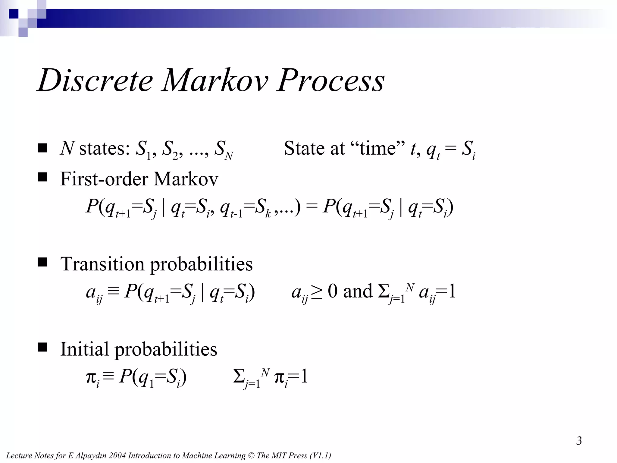
3. Discrete Markov Process N states: S 1 , S 2 , ..., S N State at “time” t , q t = S i First-order Markov P ( q t +1 = S j | q t = S i , q t -1 = S k ,...) = P ( q t +1 = S j | q t = S i ) Transition probabilities a ij ≡ P ( q t +1 = S j | q t = S i ) a ij ≥ 0 and Σ j =1 N a ij =1 Initial probabilities π i ≡ P ( q 1 = S i ) Σ j =1 N π i =1

4. Time-based Models The models typically examined by statistics: Simple parametric distributions Discrete distribution estimates These are typically based on what is called the “independence assumption”- each data point is independent of the others, and there is no time-sequencing or ordering. What if the data has correlations based on its order, like a time-series?

5. Applications of time based models Sequential pattern recognition is a relevant problem in a number of disciplines Human-computer interaction: Speech recognition Bioengineering: ECG and EEG analysis Robotics: mobile robot navigation Bioinformatics: DNA base sequence alignment

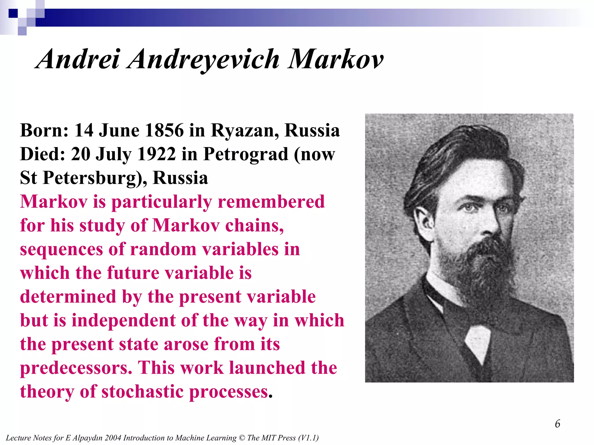
6. Andrei Andreyevich Markov Born: 14 June 1856 in Ryazan, Russia Died: 20 July 1922 in Petrograd (now St Petersburg), Russia Markov is particularly remembered for his study of Markov chains, sequences of random variables in which the future variable is determined by the present variable but is independent of the way in which the present state arose from its predecessors. This work launched the theory of stochastic processes .

7. Markov random processes A random sequence has the Markov property if its distribution is determined solely by its current state. Any random process having this property is called a Markov random process . For observable state sequences (state is known from data), this leads to a Markov chain model. For non-observable states, this leads to a Hidden Markov Model (HMM).

8. Chain Rule & Markov Property Bayes rule Markov property

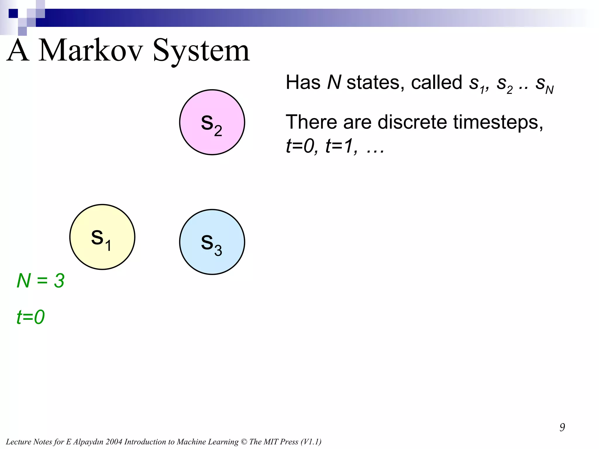
9. s 1 s 3 s 2 Has N states, called s 1 , s 2 .. s N There are discrete timesteps, t=0, t=1, … N = 3 t=0 A Markov System

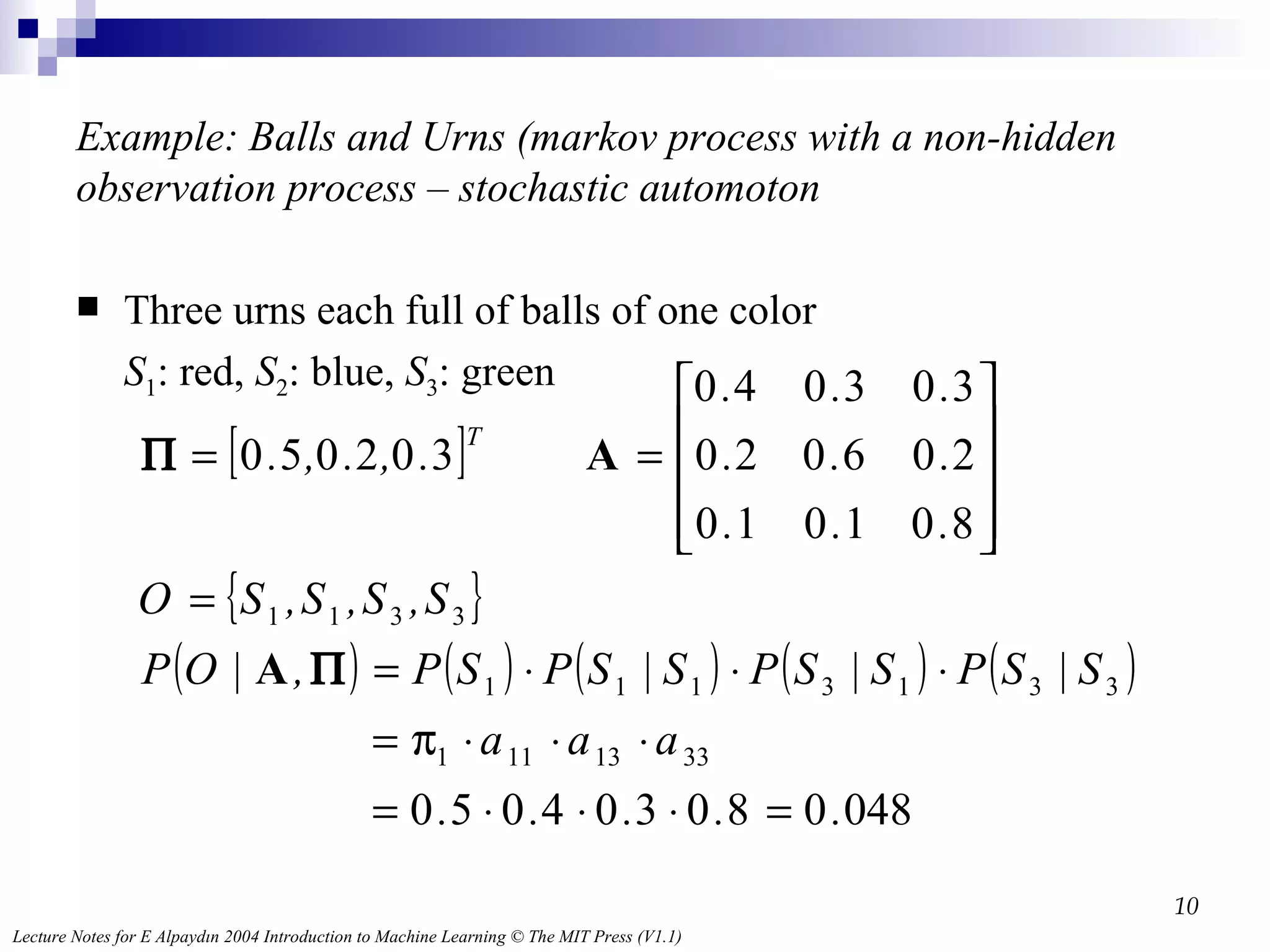
10. Example: Balls and Urns (markov process with a non-hidden observation process – stochastic automoton Three urns each full of balls of one color S 1 : red, S 2 : blue, S 3 : green

11. A Plot of 100 observed numbers for the stochastic automoton

12. Histogram for the stochastic automaton: the proportions reflect the stationary distribution of the chain

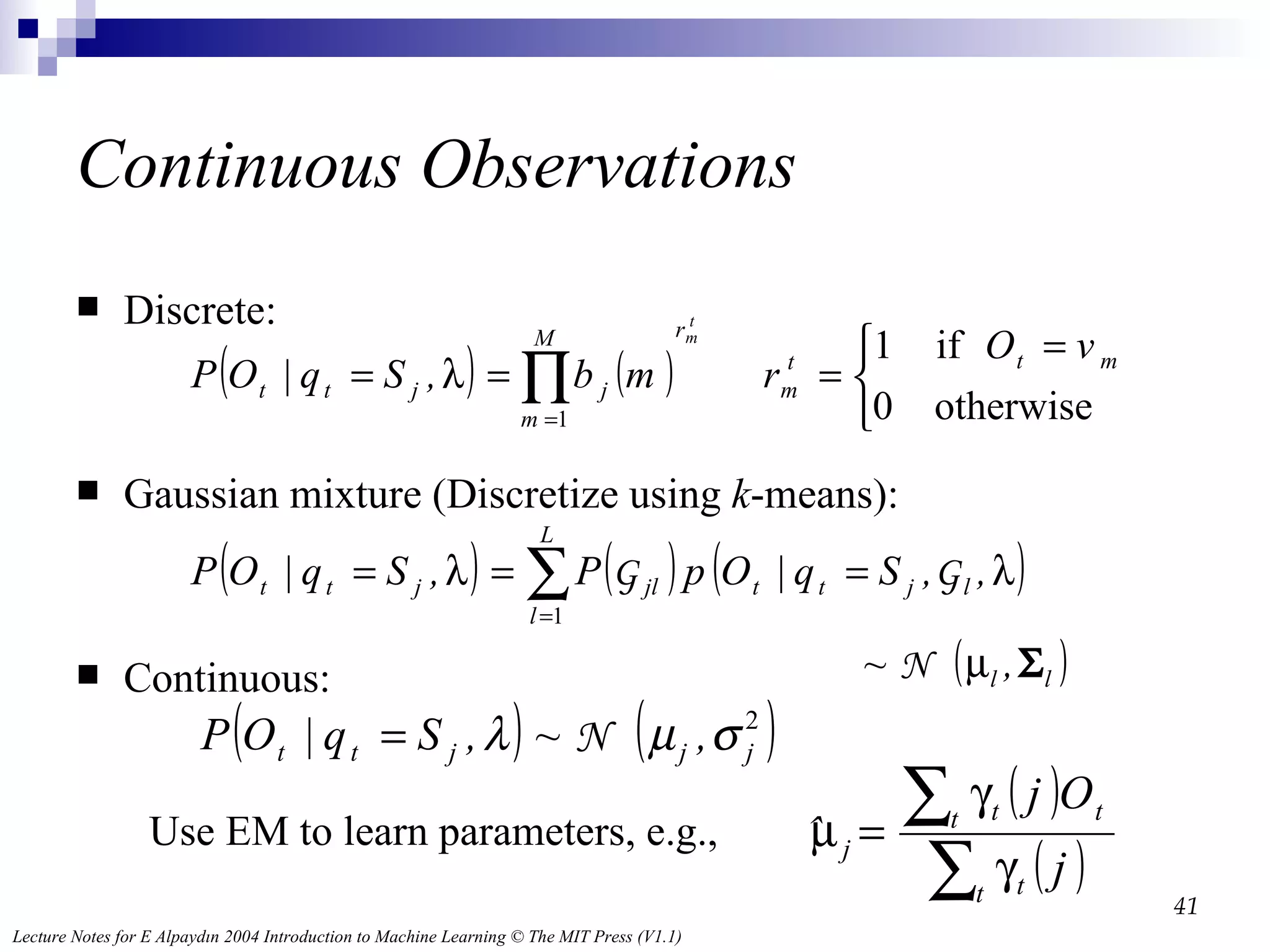
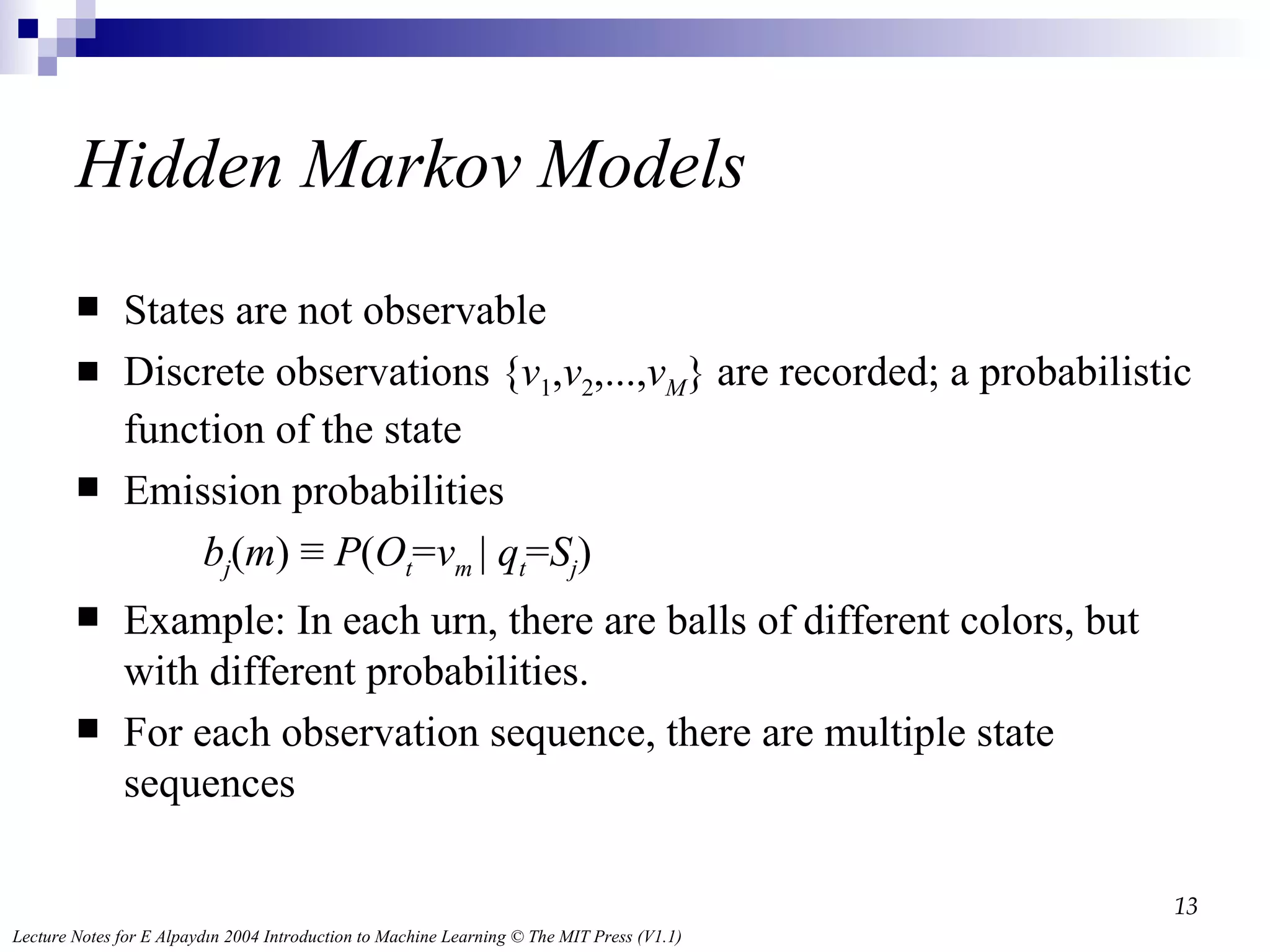
13. Hidden Markov Models States are not observable Discrete observations { v 1 , v 2 ,..., v M } are recorded; a probabilistic function of the state Emission probabilities b j ( m ) ≡ P ( O t = v m | q t = S j ) Example: In each urn, there are balls of different colors, but with different probabilities. For each observation sequence, there are multiple state sequences

14. From Markov To Hidden Markov The previous model assumes that each state can be uniquely associated with an observable event Once an observation is made, the state of the system is then trivially retrieved This model, however, is too restrictive to be of practical use for most realistic problems To make the model more flexible, we will assume that the outcomes or observations of the model are a probabilistic function of each state Each state can produce a number of outputs according to a unique probability distribution, and each distinct output can potentially be generated at any state These are known a Hidden Markov Models (HMM) , because the state sequence is not directly observable, it can only be approximated from the sequence of observations produced by the system

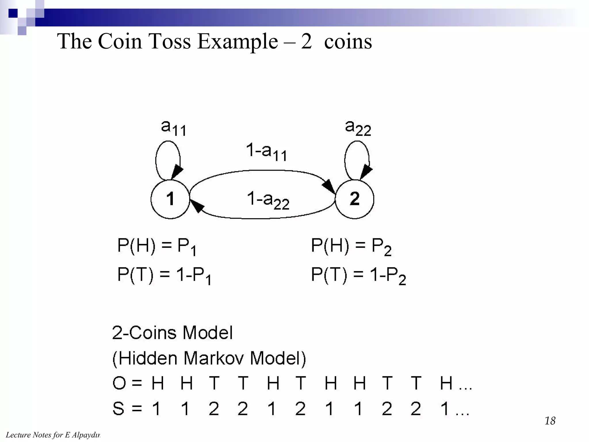
15. The coin-toss problem To illustrate the concept of an HMM consider the following scenario Assume that you are placed in a room with a curtain Behind the curtain there is a person performing a coin-toss experiment This person selects one of several coins, and tosses it: heads (H) or tails (T) The person tells you the outcome (H,T), but not which coin was used each time Your goal is to build a probabilistic model that best explains a sequence of observations O={o1,o2,o3,o4,…}={H,T,T,H,,…} The coins represent the states; these are hidden because you do not know which coin was tossed each time The outcome of each toss represents an observation A “likely” sequence of coins may be inferred from the observations, but this state sequence will not be unique

16. Speech Recognition We record the sound signals associated with words. We’d like to identify the ‘speech recognition features associated with pronouncing these words. The features are the states and the sound signals are the observations.

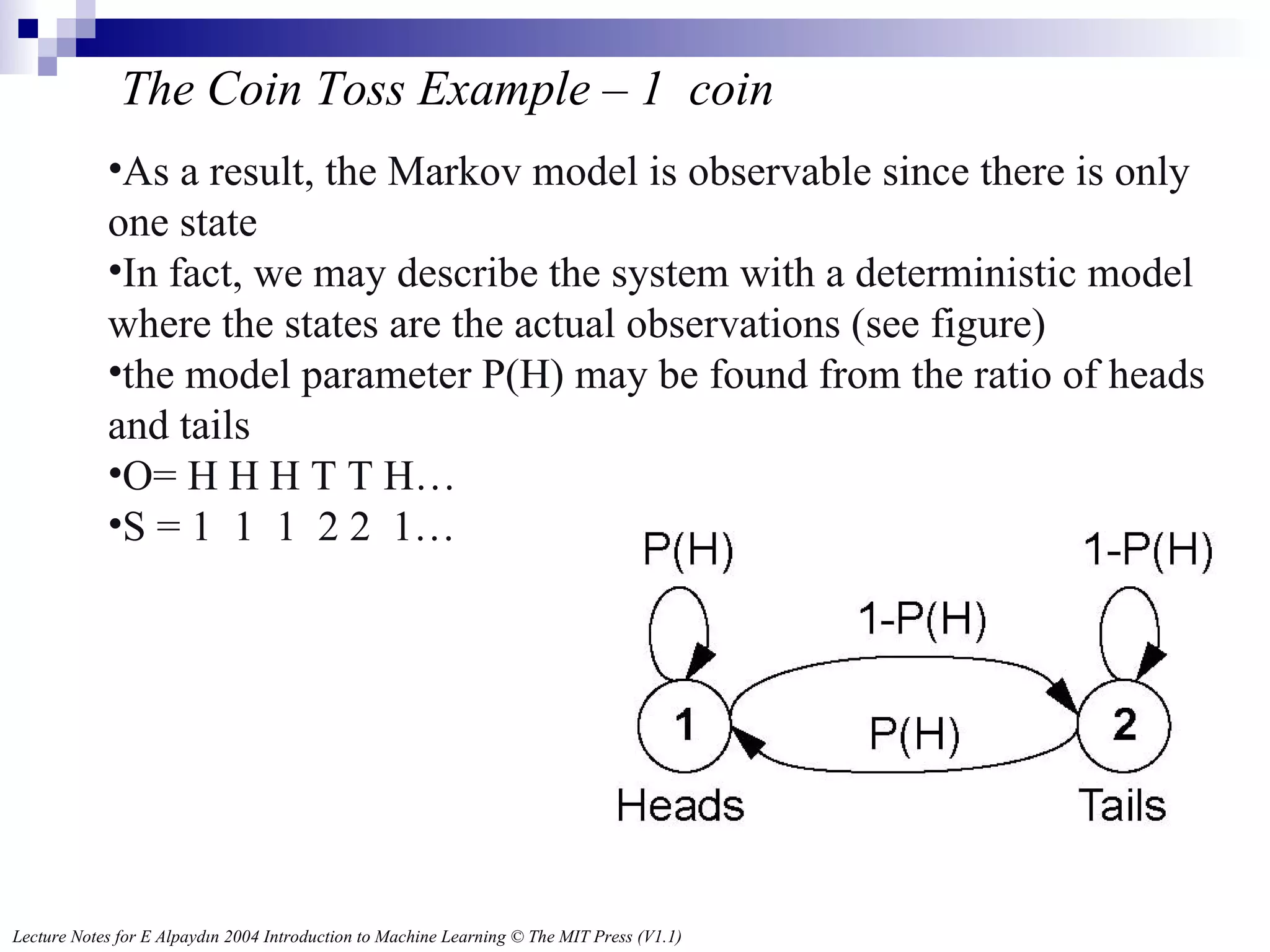
17. The Coin Toss Example – 1 coin As a result, the Markov model is observable since there is only one state In fact, we may describe the system with a deterministic model where the states are the actual observations (see figure) the model parameter P(H) may be found from the ratio of heads and tails O= H H H T T H… S = 1 1 1 2 2 1…

18. The Coin Toss Example – 2 coins

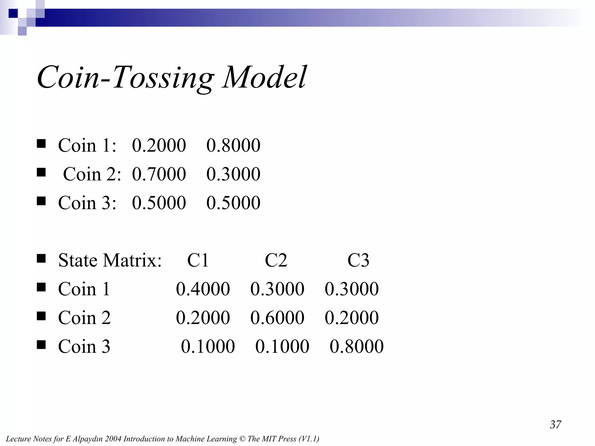
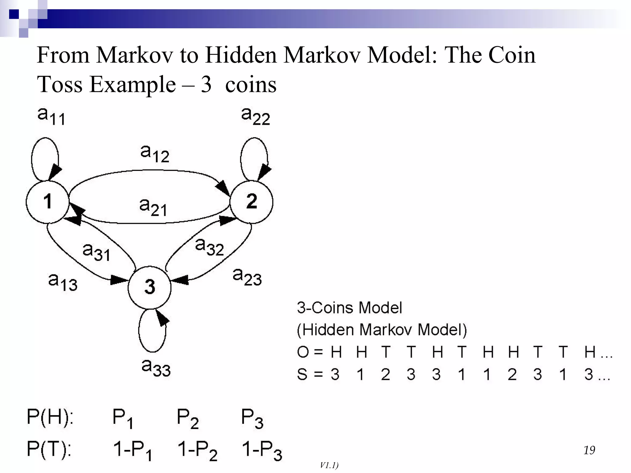
19. From Markov to Hidden Markov Model: The Coin Toss Example – 3 coins

20. 1, 2 or 3 coins? Which of these models is best? Since the states are not observable, the best we can do is select the model that best explains the data (e.g., Maximum Likelihood criterion) Whether the observation sequence is long and rich enough to warrant a more complex model is a different story, though

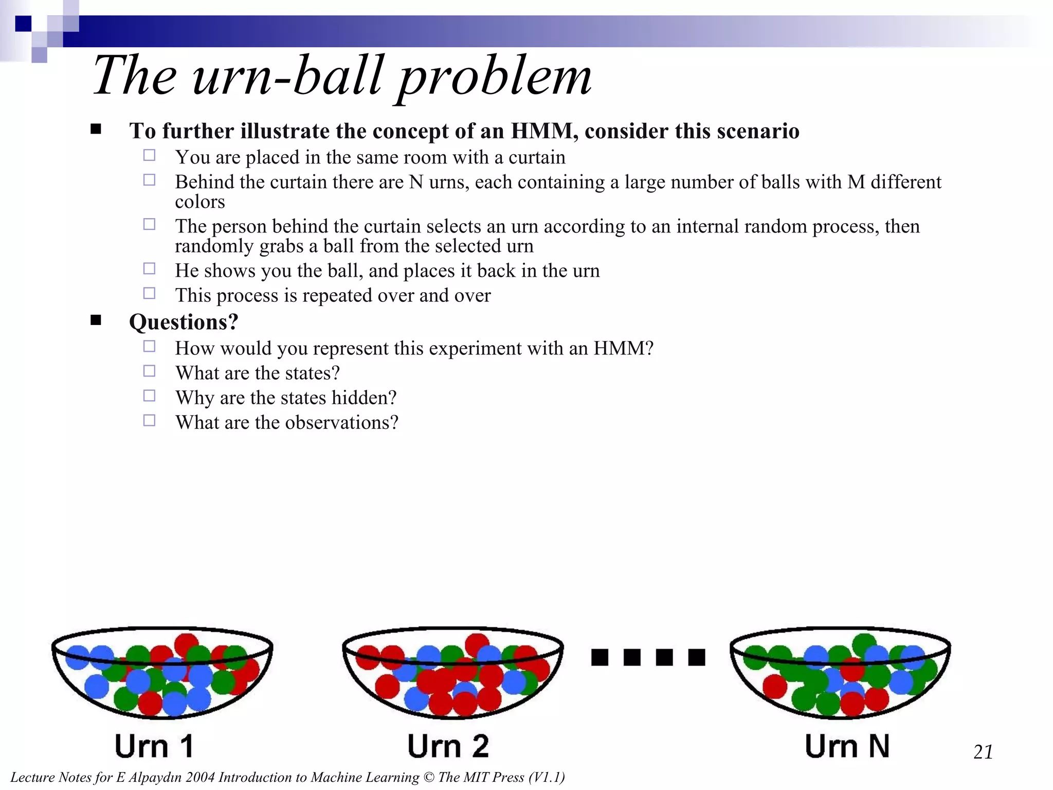
21. The urn-ball problem To further illustrate the concept of an HMM, consider this scenario You are placed in the same room with a curtain Behind the curtain there are N urns, each containing a large number of balls with M different colors The person behind the curtain selects an urn according to an internal random process, then randomly grabs a ball from the selected urn He shows you the ball, and places it back in the urn This process is repeated over and over Questions? How would you represent this experiment with an HMM? What are the states? Why are the states hidden? What are the observations?

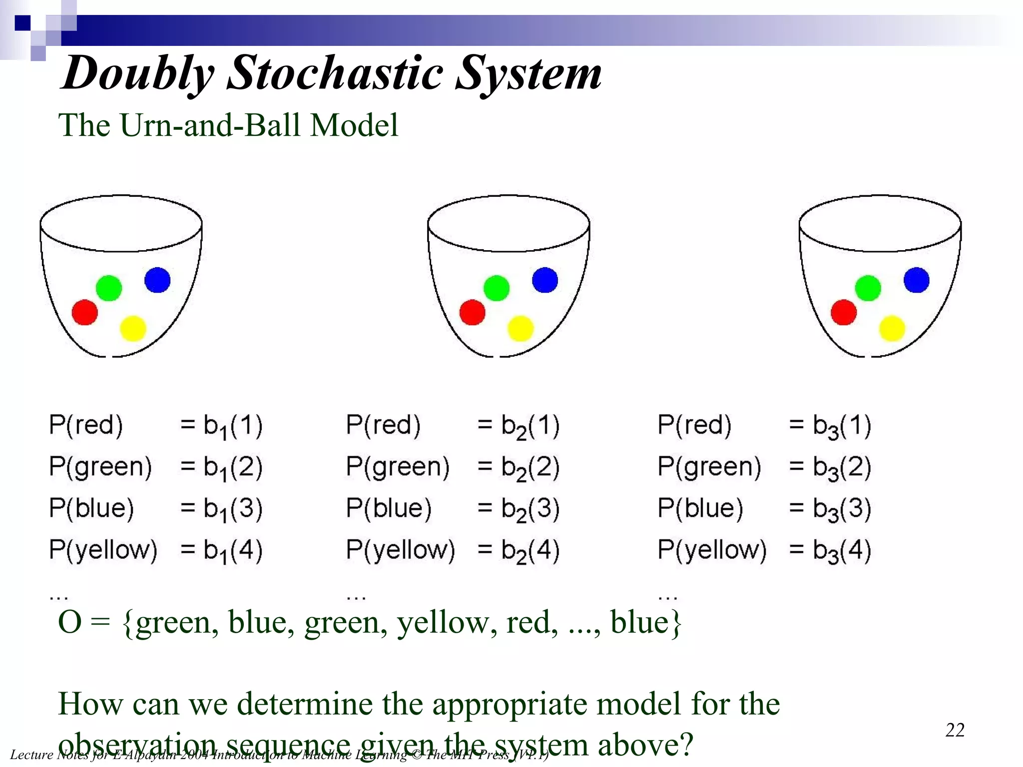
22. Doubly Stochastic System The Urn-and-Ball Model O = {green, blue, green, yellow, red, ..., blue} How can we determine the appropriate model for the observation sequence given the system above?

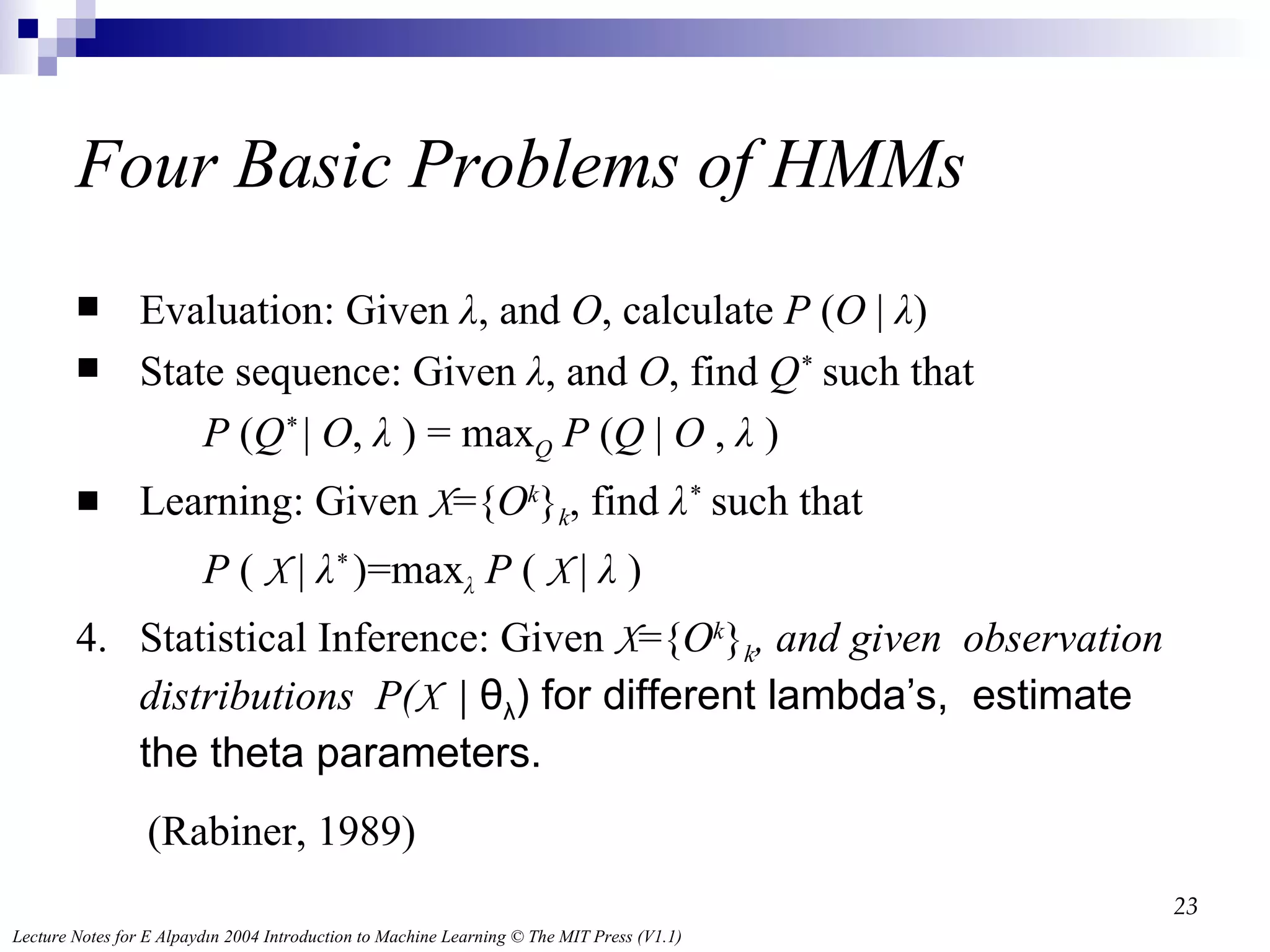
23. Four Basic Problems of HMMs Evaluation: Given λ , and O , calculate P ( O | λ ) State sequence: Given λ , and O , find Q * such that P ( Q * | O , λ ) = max Q P ( Q | O , λ ) Learning: Given X ={ O k } k , find λ * such that P ( X | λ * )=max λ P ( X | λ ) 4. Statistical Inference : Given X ={ O k } k , and given observation distributions P( X | θ λ ) for different lambda’s, estimate the theta parameters. (Rabiner, 1989)

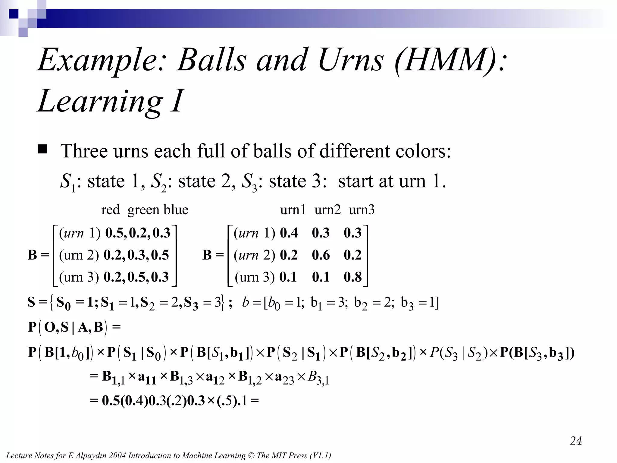
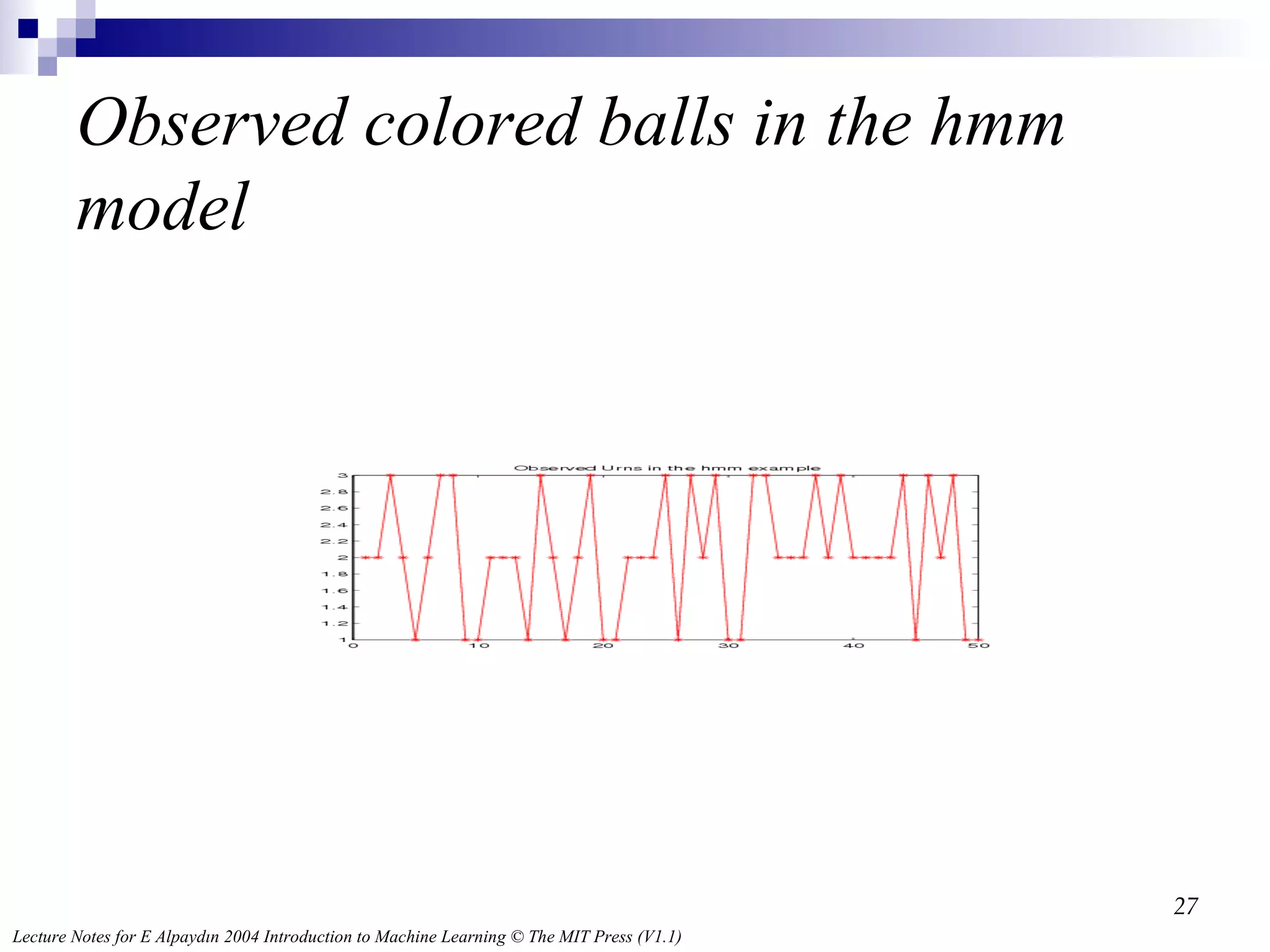
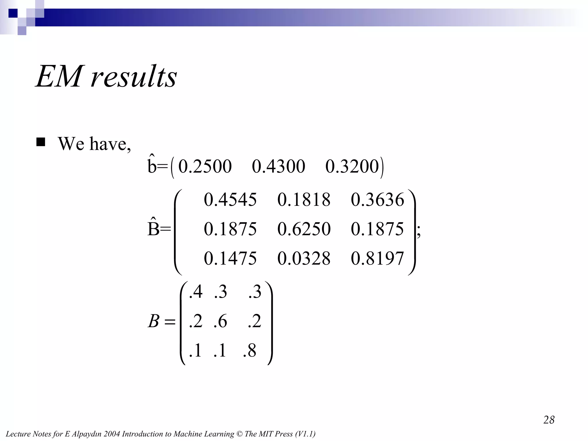
24. Example: Balls and Urns (HMM): Learning I Three urns each full of balls of different colors: S 1 : state 1 , S 2 : state 2 , S 3 : state 3: start at urn 1.

25. Baum-Welch EM for Hidden Markov Models We use the notation q t for the probability of the result at time t; a i[t-1],i[t] for the probability of going from the observed state at time t-1 to the observed state at time t; n i for the observed number of results i, and n i,j for the number of transitions from I to j;

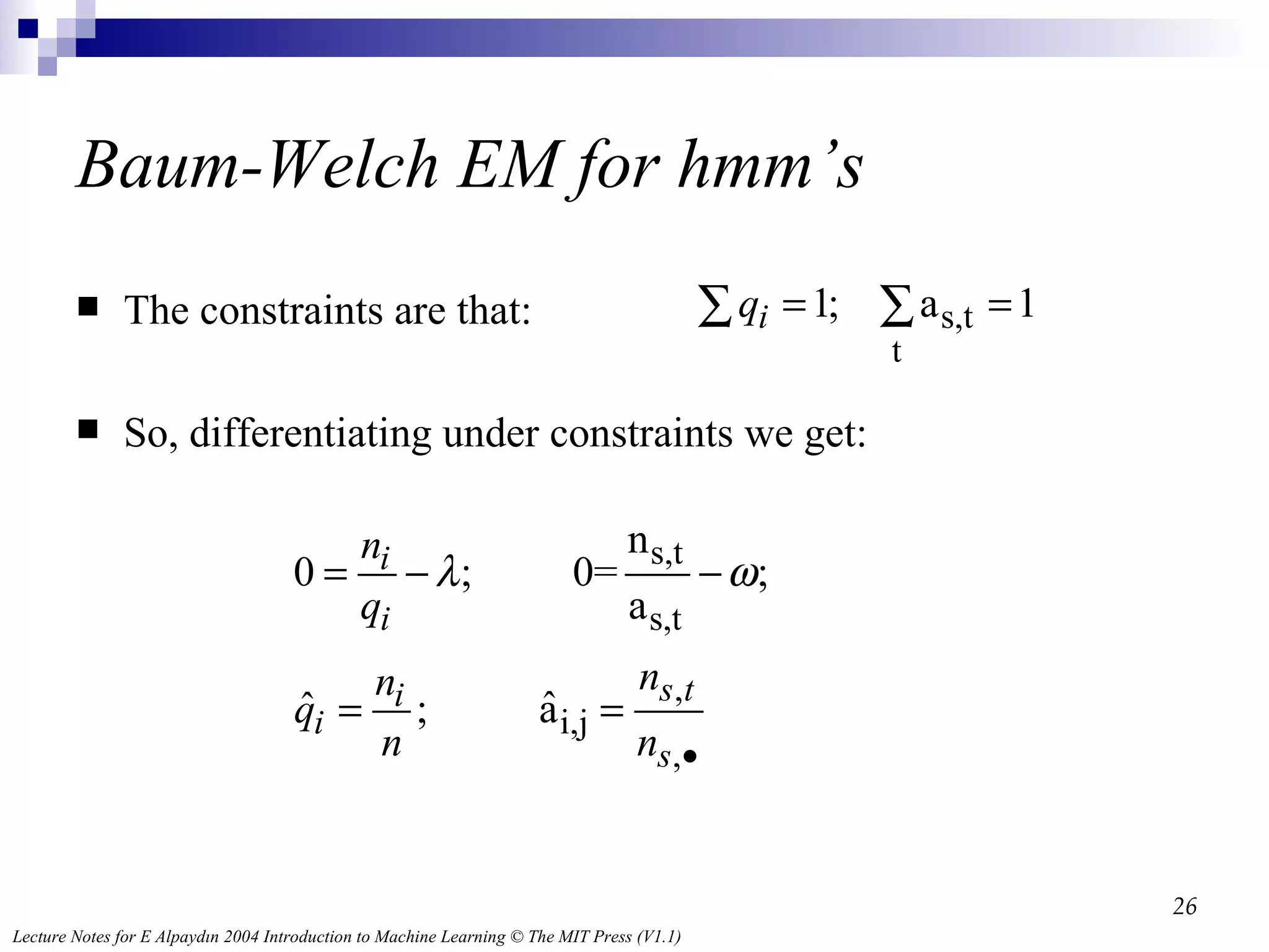
26. Baum-Welch EM for hmm’s The constraints are that: So, differentiating under constraints we get:

27. Observed colored balls in the hmm model

28. EM results We have,

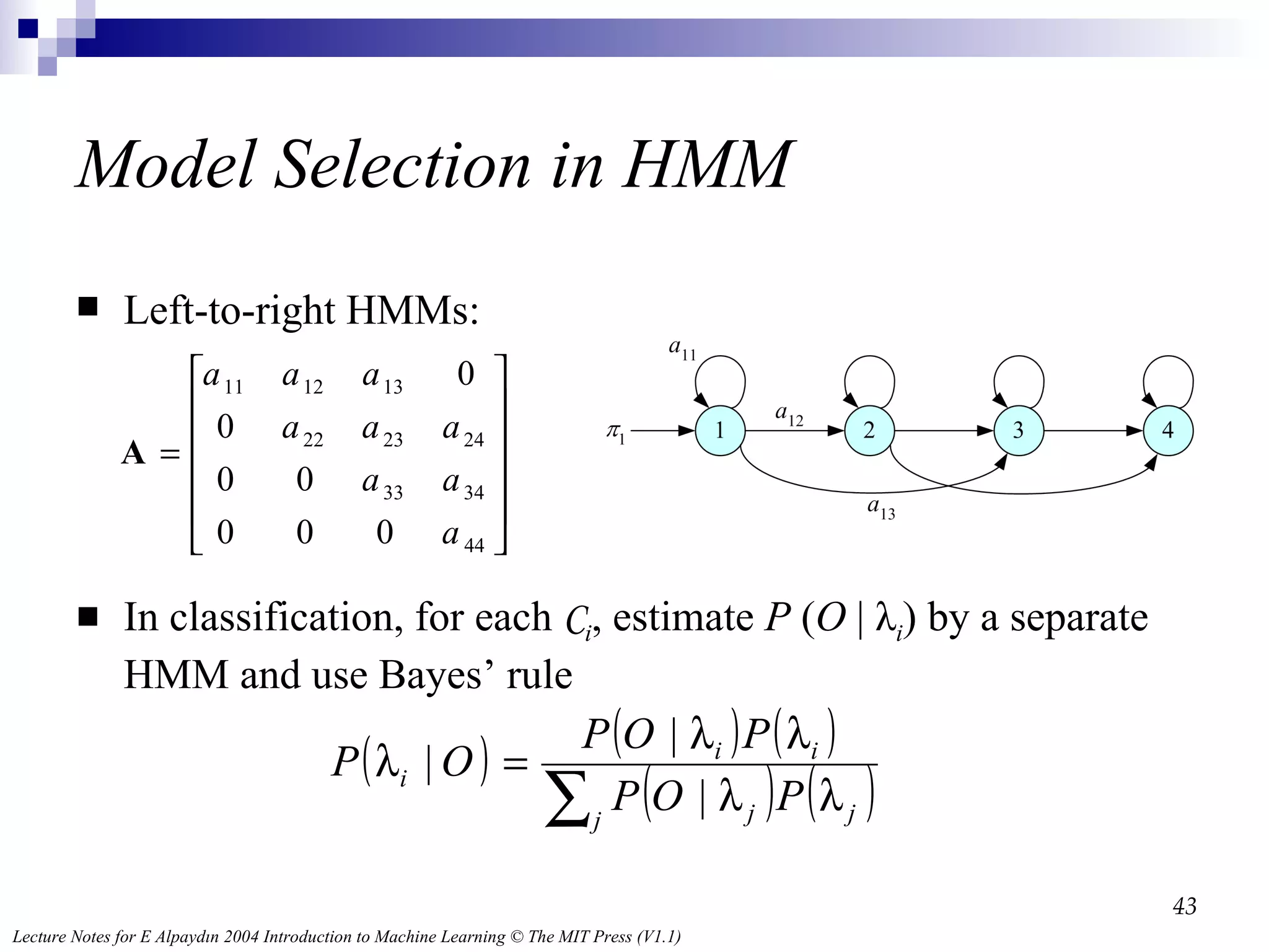
29. More General Elements of an HMM N : Number of states M : Number of observation symbols A = [ a ij ]: N by N state transition probability matrix B = b j (m) : N by M observation probability matrix Π = [ π i ]: N by 1 initial state probability vector λ = ( A , B , Π ), parameter set of HMM

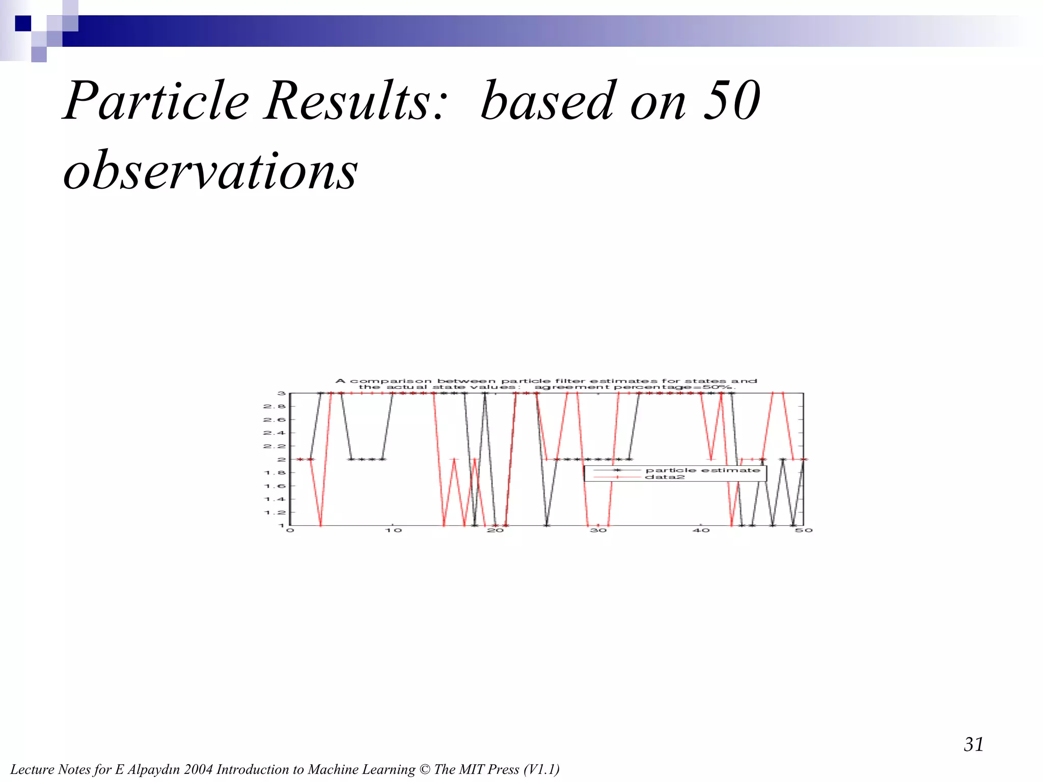
30. Particle Evaluation At stage t, simulate the new state from the former state using the distribution, and Weight the result by, . The resulting weight for the j’th particle is: We should use standard residual resampling. The result gets 50 percent accuracy [Note: I haven’t perfected good residual sampling].

31. Particle Results: based on 50 observations

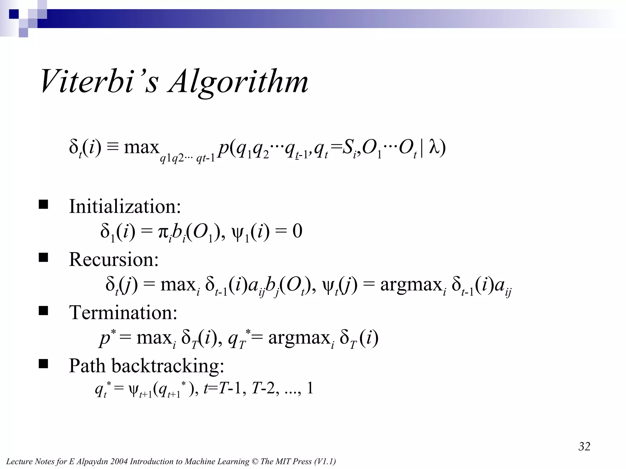
32. Viterbi’s Algorithm δ t ( i ) ≡ max q 1 q 2∙∙∙ qt -1 p ( q 1 q 2 ∙∙∙ q t -1 ,q t = S i , O 1 ∙∙∙ O t | λ) Initialization: δ 1 ( i ) = π i b i ( O 1 ), ψ 1 ( i ) = 0 Recursion: δ t ( j ) = max i δ t -1 ( i ) a ij b j ( O t ), ψ t ( j ) = argmax i δ t -1 ( i ) a ij Termination: p * = max i δ T ( i ), q T * = argmax i δ T ( i ) Path backtracking: q t * = ψ t +1 ( q t +1 * ), t = T -1, T -2, ..., 1

33. Viterbi learning versus the actual state (estimate =3; 62% accuracy)

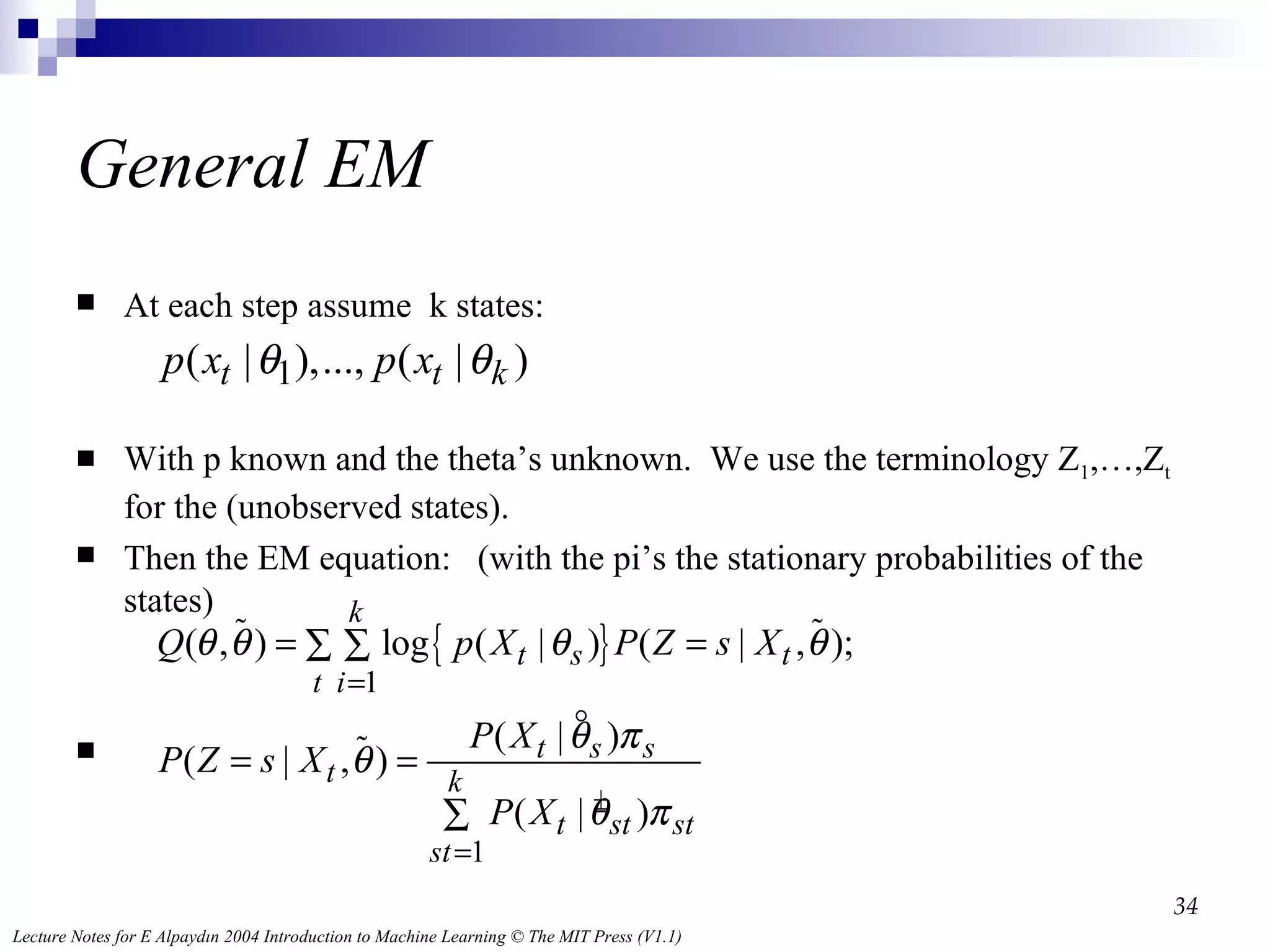
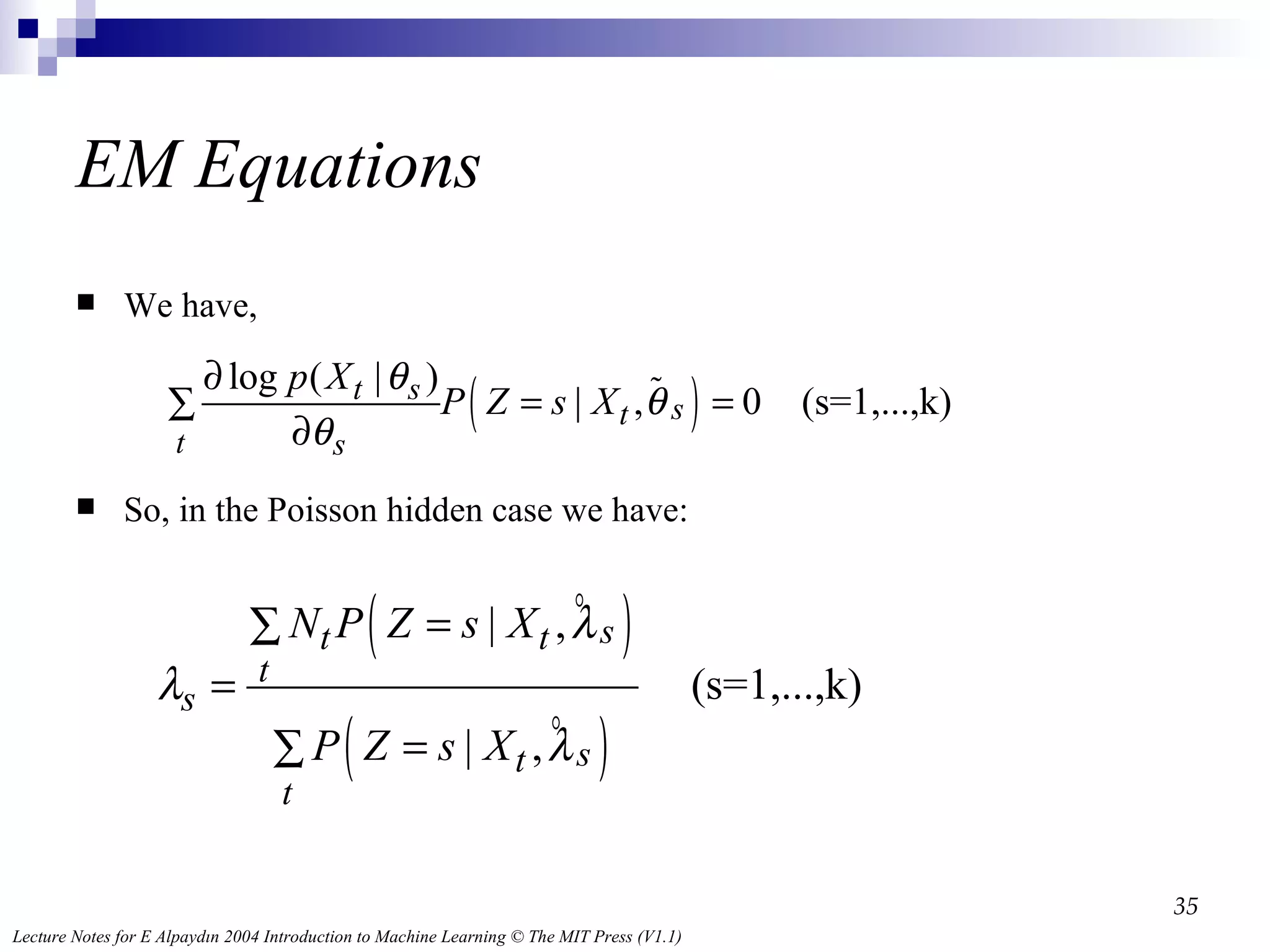
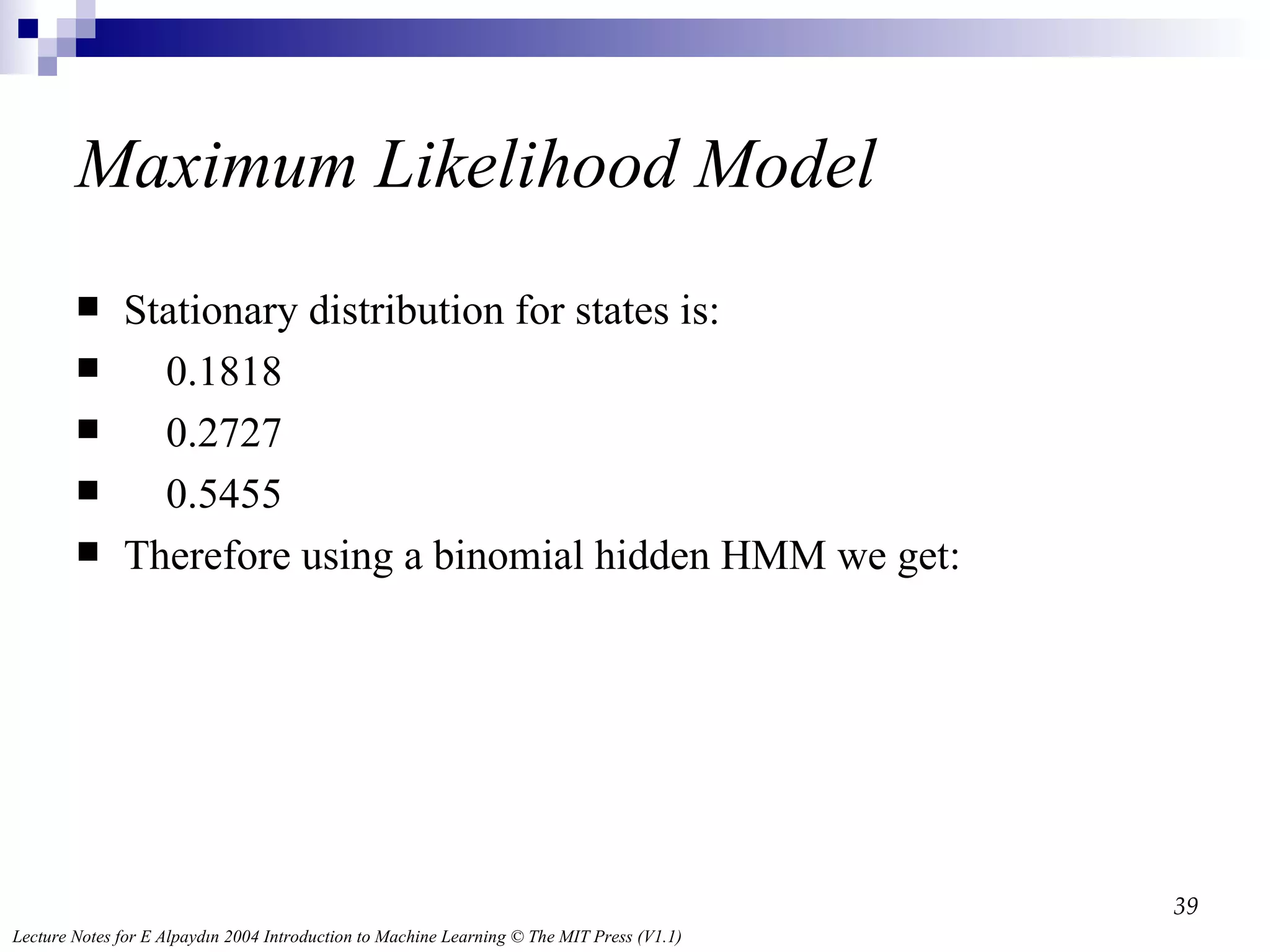
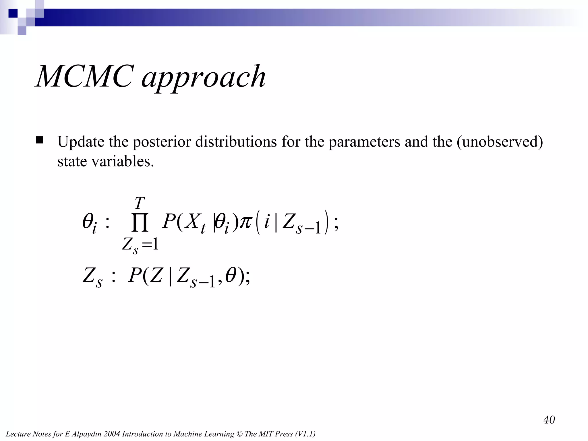
34. General EM At each step assume k states: With p known and the theta’s unknown. We use the terminology Z 1 ,…,Z t for the (unobserved states). Then the EM equation: (with the pi’s the stationary probabilities of the states)

35. EM Equations We have, So, in the Poisson hidden case we have:

36. Binomial hidden model We have:

37. Coin-Tossing Model Coin 1: 0.2000 0.8000 Coin 2: 0.7000 0.3000 Coin 3: 0.5000 0.5000 State Matrix: C1 C2 C3 Coin 1 0.4000 0.3000 0.3000 Coin 2 0.2000 0.6000 0.2000 Coin 3 0.1000 0.1000 0.8000

38. Coin tossing model: results

39. Maximum Likelihood Model Stationary distribution for states is: 0.1818 0.2727 0.5455 Therefore using a binomial hidden HMM we get:

40. MCMC approach Update the posterior distributions for the parameters and the (unobserved) state variables.

41. Continuous Observations Discrete: Gaussian mixture (Discretize using k -means): Continuous: Use EM to learn parameters, e.g.,

42. HMM with Input Input-dependent observations: Input-dependent transitions (Meila and Jordan, 1996; Bengio and Frasconi, 1996): Time-delay input:

43. Model Selection in HMM Left-to-right HMMs: In classification, for each C i , estimate P ( O | λ i ) by a separate HMM and use Bayes’ rule