Download as PDF, PPTX


![Movements
and
Performance
Metulini,
Manisera,
Zuccolotto
Context
Data
Methods &
Results
Conclusions
Acknowledgm.
& References
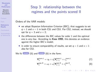
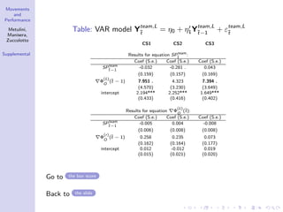
Step 3: relationship between the
regimes and the points scored
SPteam
¯t and SPopp
¯t
: points scored by the team and the opponents, in the
time interval (¯t − 1,¯t], where ¯t = 1, 2, · · · ,¯t express minutes.
Yteam,L
¯t
and Yopp,N
¯t
are the vectors
Yteam,L
¯t
=
SPteam
¯t
ΦL
O(¯t)
and Yopp,N
¯t
=
SPopp
¯t
ΦN
D(¯t)
, (4)
We assume a VAR model (Sims 1980):
Yteam,L
¯t
= η0 + η1Yteam,L
¯t−1
+ · · · + ηqYteam,L
¯t−q
+ εteam,L
¯t
(5)
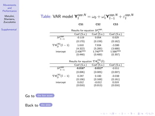
Yopp,N
¯t
= ω0 + ω1Yopp,N
¯t−1
+ · · · + ωs Yopp,N
¯t−s
+ εopp,N
¯t
, (6)
η0, ω0: 2 × 1 vectors of the intercepts,
η1 ... ηq, ω1 ... ωs : 2 × 2 matrices of the coefficients,
εteam,L
¯t
, εopp,N
¯t
are the innovation processes.](https://image.slidesharecdn.com/metulini280818iasi-180903102047/85/Metulini280818-iasi-15-320.jpg)


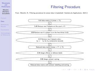
The document discusses the modeling of dynamic patterns of surface area in basketball and their impact on team performance using statistical methods. It aims to analyze how player positioning affects both offensive and defensive plays, employing a Markov switching model and various data processing techniques. The findings indicate differing regime behaviors during different phases of the game and suggest avenues for further research on player trajectories and tactical influences.


