For any help regarding Stochastic Processes Assignment Help
Visit : https://www.statisticsassignmenthelp.com/ ,
Email - info@statisticsassignmenthelp.com or
Call us at - +1 678 648 4277
Solution to Exercise 2.28:
The purpose of this problem is to illustrate that for an arrival process with
independent but not identically distributed interarrival intervals, X1,X2,...,, the
number of arrivals N(t) in the interval (0,t] can be a defective rv. In other words,
the ‘counting process’ is not a stochastic process according to our definitions. This
illustrates that it is necessary to prove that the counting rv’s for a renewal
process are actually rv’s.
a) Let the distribution function of the ith interarrival interval for an arrival
process be FXi (x i) = 1 − exp(−α− xi) for some fixed α ∈ (0, 1). Let Sn = X1 + ··· Xn
and show that
b) Sketch a ‘reasonable’ sample function for N(t).
c) Find σ2 Sn .
d) Use the Chebyshev inequality on Pr Sn ≥ t to find an upper bound on Pr N(t)
≤ n that is smaller than 1 for all n and for large enough t. Use this to show
that N(t) is defective for large enough t.
SOLUTION: a) Each Xi is an exponential rv, of rate αi, so E[Xi] = αi . Thus
statisticsassignmenthelp.com
Recalling that 1 + α + α2 + ··· = 1/(1 − α),
In other words, not only is E[Xi] decaying to 0 geometrically with increasing i,
but E[Sn] is upper bounded, for all n, by α/(1 − α).
b) Since the expected interarrival times are decaying geometrically and the
expected arrival epochs are bounded for all n, it is reasonable for a sample path
to have the following shape:
Note that the question here is not precise (there are obviously many sample paths, and
which are ‘reasonable’ is a matter of interpretation). The reason for drawing such
sketches is to acquire understanding to guide the solution to the following parts of the
problem. c) Since Xi is exponential, σ2= α2i X. Since the Xi i are independent,
statisticsassignmenthelp.com
d) The figure suggests (but does not prove) that for typical sample functions (and in
particular for a set of sample functions of nonzero probability), N(t) goes to infinity for
finite values of t. If the probability that N(t) ≤ n (for a given t) is bounded, independent
of n, by a number strictly less than 1, then that N(t) is a defective rv rather than a true
rv.
The problem suggests using the Chebyshev bound to prove this, but the Markov
bound is both simpler and also shows that N(t) is defective for smaller values of t than
established by Chebyshev. Thus we first use Markov and then use Chebyshev. By
Markov,
where we have used Eq. 2.3 in the text. Since this is valid for all n, it is also valid for Pr
N(t) ≤ n. For any t > α/(1 − α), we see that α< 1. Thus N(t) is defective for t(1−α)
anysuch t, i.e., for any t greater than limn→∞ ESn.
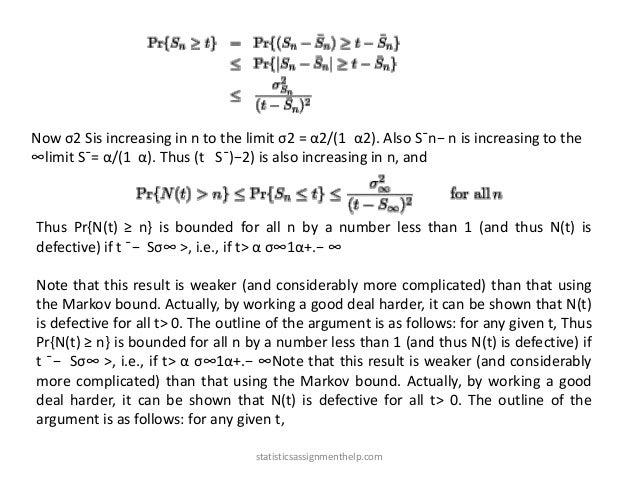
Now to use Chebyshev, note that
statisticsassignmenthelp.com
Now σ2 Sis increasing in n to the limit σ2 = α2/(1 α2). Also S¯n− n is increasing to the
∞limit S¯= α/(1 α). Thus (t S¯)−2) is also increasing in n, and
Thus Pr{N(t) ≥ n} is bounded for all n by a number less than 1 (and thus N(t) is
defective) if t ¯− Sσ∞ >, i.e., if t> α σ∞1α+.− ∞
Note that this result is weaker (and considerably more complicated) than that using
the Markov bound. Actually, by working a good deal harder, it can be shown that N(t)
is defective for all t> 0. The outline of the argument is as follows: for any given t, Thus
Pr{N(t) ≥ n} is bounded for all n by a number less than 1 (and thus N(t) is defective) if
t ¯− Sσ∞ >, i.e., if t> α σ∞1α+.− ∞Note that this result is weaker (and considerably
more complicated) than that using the Markov bound. Actually, by working a good
deal harder, it can be shown that N(t) is defective for all t> 0. The outline of the
argument is as follows: for any given t,
statisticsassignmenthelp.com
Solution to Exercise 3.2:
a) Based on the definition of the recurrent states, if a state is accessible from all
the states that are accessible from it, (i.e., if for all i2 that i1 → i2, we also
have i2 → i1), the state i1 is called recurrent. So if a state is not recurrent
(i.e., it is transient), there should exist at least one state i2 that is accessible
from i1 (i1 → i2) but i1 is not accessible from it (i2 i1).
b) The same reasoning as in part (a) shows that if i2 is transient, there should
exist a state i3 where i2 → i3 but i3 i2. Additionally, we know that i1 → i2
and i2 → i3 imply that i1 → i3.
We know that i1 → i2. Now if i3 → i1, then i3 → i2 which is against what
we said about i3. Then i1 should not be accessible from i3. (i.e., i3 i1)
c) The same reasoning as in part (a) shows that if ik is transient, there should
exist a state ik+1 for which ik → ik+1 but ik+1 ik. Now if for any 1 ≤ j ≤ k,
ik+1 → j, then we also have ik+1 → ik which is against the assumption about
ik.
d) Each state ik constructed in part c) is distinct from states i1,...,ik 1, since there
is − a path from ij to ik but not from ik to ij . Since there are only J states,
the process in part c) must terminate with some k ≤ J, with means that ik
isn’t transient, i.e., is recurrent.
statisticsassignmenthelp.com
Solution to Exercise 3.3:
In exercise 3.2 it is proved that each Markov chain has at least one recurrent
state which induces a recurrent class of states. State 1 is accessible from all
the states. So it is also accessible from the states of the recurrent class in this
Markov chain. According to the definition of recurrent class, all the states that
are accessible from the states of a recurrent class should have access to the
states of this class, meaning that state 1 should communi cate to all of the
classes of recurrent states. If two recurrent states communicate with one state,
they should also communicate with each other, i.e., they belong to a single
recurrent class. Hence, there should exist at most one recurrent class of states
in this Markov chain.
Problem 4:
The desired graph is shown below. It should be clear that this construction can
be used for any number of states M ≥ 3. Starting in state 1, there is only one
possible state (first 2, then 3, up to J) that the chain can be for the first J − 1
steps. On the Jth step, there are two possible states (1 and 2). For each step
from M to 2M − 2, there are two possible states (first 1,2, then 2,3, up to M
− 1,M. Similarly, from steps 2(M − 1) + 1 to 3(M − 1), there are 3 possible
states (first 1, 2, 3, then 2, 3, 4, etc.). This continues up to (M − 1)2, which is
the last step at which there are M 1 possible states, and then from ( − + 1
on, all states are possible at each transition.
statisticsassignmenthelp.com
This pattern should be clear from your tabulation for M = 4. The desired graph
is shown below. It should be clear that this construction exists for all J ≥ 3.
Any walk from node J back to node J must be of length iJ + k(J − 1) for some
i ≥ 1 and some k ≥ 1. Note that iJ + k(J − 1) = i +(i + k)(J − 1). Trying to set this
equal to (J − 1)2 yields i + (i + k − J + 1)(J − 1) = 0. This implies that i is a
multiple J − 1, which makes iJ > (J − 1)2, so there is no walk from node J back
to itself in (J − 1)2 steps.
Solution to Exercise 3.8:
[P ] is doubly stochastic if both [P ] and [P ]T are stochastic. This is just a
different way of saying that all the rows and all the columns of [P ] must sum
to one (and all entries are non-negative). Since [P ] is stochastic, it has e (a
column vector) as a right eigenvector with the associated eigenvalue λ = 1,
i.e., [P ]e = e. Since [ P ]T is stochastic also, [P ]Te = e. Taking transposes of
both sides we get eT [P ] = eT , so eT is a left eigenvector of [P ] asso ciated
with λ = 1. Theorem 3.3.1 guarantees that this left eigenvector is unique
within a scale factor, so scaling eT to become a probability vector, π = [1/M,
1/M/, ··· , 1/M]. statisticsassignmenthelp.com
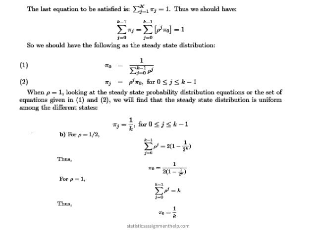
Solution to Exercise 3.9: a) K The steady state distribution of the Markov chain.
is a probability vector π for which j=1 πj = 1 and for each 1 ≤ j ≤ K, πj = i=1
Pij πi. In this Markov chain, We can have the following equations:
From the first equations we can have:
Using the second equation and π1 = pπ0
The last equation says = pππ. ρ = pk1 Calling, 1for 0 j k 1 we should −−p k−21−p
≤≤−have:
statisticsassignmenthelp.com
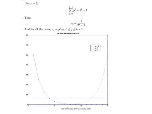
As you observe ρ can be considered as a measure of flow among the states in
the Markov chain. When ρ < 1, the flow is towards left and the state 0 has the
highest probability. When ρ > 1, the flow is towards right and the state k−1 has
the highest probability. When ρ = 1, there is no flow in any specific direction
and the steady state distribution is uniform.
c) If ρ = 1, we have:
So if ρ< 1, as k →∞, π0 → 1 − ρ and πk−1 → 0. And if ρ> 1, as k →∞, π0 → 0 and
πk−1 → 1 − 1/ρ. For ρ = 1, the steady state distribution is uniform and π0 = πk−1
=1/k → 0. For ρ< 1, the PMF drops off geometrically with ρ, the process returns to
the zero state often and rarely wanders off to the higher states. Taking the limit,
limk π=→∞0 (1 − ρ), limk πk1 = 0. For ρ = 1, all probabilities are equal, and limk π0
= 0, →∞−→∞limk πk1 = 0. For ρ> 1, the probabilities increase with i and as k gets
larger, →∞−it is increasingly unlikely to be in state 0. Taking the limits, limk→∞ π0 =
(1 − ρ), limk→∞ πk−1 = 0.
statisticsassignmenthelp.com
Solution to Exercise 3.10:
a) The transition matrix of the first graph is:
The steady state distribution will satisfy the following equations:
Solving these set of equations, we get:
This was almost obvious considering the symmetry of the graph and equations.
statisticsassignmenthelp.com
b)
Let’s define q =2p(1 − p). Then the corresponding Markov chain to [P1]2 is:You can
observe that as the original Markov chain is periodic with period d =2, [P ]d partitions
the Markov chain into d disjoint recurrent classes.
Since, [P ]2 has two recurrent classes, there are two independent steady state
distributions for this Markov chain.
statisticsassignmenthelp.com
Any linear combination of these steady state distributions is also a steady state
distribution of this Markov chain. c) If the initial state of the Markov chain is 1 or 3,
i.e., X0 ∈{1, 3}, the steady state distribution at time 2n as n →∞, is [1/2, 0, 1/2, 0]. If
the initial state of the Markov chain is 2 or 4, i.e., X0 ∈{2, 4}, the steady state
distribution at time 2n as n →∞, is [0, 1/2, 0, 1/2]. Thus we will have:
statisticsassignmenthelp.com

Stochastic Processes Assignment Help

  • 1.
    For any helpregarding Stochastic Processes Assignment Help Visit : https://www.statisticsassignmenthelp.com/ , Email - info@statisticsassignmenthelp.com or Call us at - +1 678 648 4277
  • 2.
    Solution to Exercise2.28: The purpose of this problem is to illustrate that for an arrival process with independent but not identically distributed interarrival intervals, X1,X2,...,, the number of arrivals N(t) in the interval (0,t] can be a defective rv. In other words, the ‘counting process’ is not a stochastic process according to our definitions. This illustrates that it is necessary to prove that the counting rv’s for a renewal process are actually rv’s. a) Let the distribution function of the ith interarrival interval for an arrival process be FXi (x i) = 1 − exp(−α− xi) for some fixed α ∈ (0, 1). Let Sn = X1 + ··· Xn and show that b) Sketch a ‘reasonable’ sample function for N(t). c) Find σ2 Sn . d) Use the Chebyshev inequality on Pr Sn ≥ t to find an upper bound on Pr N(t) ≤ n that is smaller than 1 for all n and for large enough t. Use this to show that N(t) is defective for large enough t. SOLUTION: a) Each Xi is an exponential rv, of rate αi, so E[Xi] = αi . Thus statisticsassignmenthelp.com
  • 3.
    Recalling that 1+ α + α2 + ··· = 1/(1 − α), In other words, not only is E[Xi] decaying to 0 geometrically with increasing i, but E[Sn] is upper bounded, for all n, by α/(1 − α). b) Since the expected interarrival times are decaying geometrically and the expected arrival epochs are bounded for all n, it is reasonable for a sample path to have the following shape: Note that the question here is not precise (there are obviously many sample paths, and which are ‘reasonable’ is a matter of interpretation). The reason for drawing such sketches is to acquire understanding to guide the solution to the following parts of the problem. c) Since Xi is exponential, σ2= α2i X. Since the Xi i are independent, statisticsassignmenthelp.com
  • 4.
    d) The figuresuggests (but does not prove) that for typical sample functions (and in particular for a set of sample functions of nonzero probability), N(t) goes to infinity for finite values of t. If the probability that N(t) ≤ n (for a given t) is bounded, independent of n, by a number strictly less than 1, then that N(t) is a defective rv rather than a true rv. The problem suggests using the Chebyshev bound to prove this, but the Markov bound is both simpler and also shows that N(t) is defective for smaller values of t than established by Chebyshev. Thus we first use Markov and then use Chebyshev. By Markov, where we have used Eq. 2.3 in the text. Since this is valid for all n, it is also valid for Pr N(t) ≤ n. For any t > α/(1 − α), we see that α< 1. Thus N(t) is defective for t(1−α) anysuch t, i.e., for any t greater than limn→∞ ESn. Now to use Chebyshev, note that statisticsassignmenthelp.com
  • 5.
    Now σ2 Sisincreasing in n to the limit σ2 = α2/(1 α2). Also S¯n− n is increasing to the ∞limit S¯= α/(1 α). Thus (t S¯)−2) is also increasing in n, and Thus Pr{N(t) ≥ n} is bounded for all n by a number less than 1 (and thus N(t) is defective) if t ¯− Sσ∞ >, i.e., if t> α σ∞1α+.− ∞ Note that this result is weaker (and considerably more complicated) than that using the Markov bound. Actually, by working a good deal harder, it can be shown that N(t) is defective for all t> 0. The outline of the argument is as follows: for any given t, Thus Pr{N(t) ≥ n} is bounded for all n by a number less than 1 (and thus N(t) is defective) if t ¯− Sσ∞ >, i.e., if t> α σ∞1α+.− ∞Note that this result is weaker (and considerably more complicated) than that using the Markov bound. Actually, by working a good deal harder, it can be shown that N(t) is defective for all t> 0. The outline of the argument is as follows: for any given t, statisticsassignmenthelp.com
  • 6.
    Solution to Exercise3.2: a) Based on the definition of the recurrent states, if a state is accessible from all the states that are accessible from it, (i.e., if for all i2 that i1 → i2, we also have i2 → i1), the state i1 is called recurrent. So if a state is not recurrent (i.e., it is transient), there should exist at least one state i2 that is accessible from i1 (i1 → i2) but i1 is not accessible from it (i2 i1). b) The same reasoning as in part (a) shows that if i2 is transient, there should exist a state i3 where i2 → i3 but i3 i2. Additionally, we know that i1 → i2 and i2 → i3 imply that i1 → i3. We know that i1 → i2. Now if i3 → i1, then i3 → i2 which is against what we said about i3. Then i1 should not be accessible from i3. (i.e., i3 i1) c) The same reasoning as in part (a) shows that if ik is transient, there should exist a state ik+1 for which ik → ik+1 but ik+1 ik. Now if for any 1 ≤ j ≤ k, ik+1 → j, then we also have ik+1 → ik which is against the assumption about ik. d) Each state ik constructed in part c) is distinct from states i1,...,ik 1, since there is − a path from ij to ik but not from ik to ij . Since there are only J states, the process in part c) must terminate with some k ≤ J, with means that ik isn’t transient, i.e., is recurrent. statisticsassignmenthelp.com
  • 7.
    Solution to Exercise3.3: In exercise 3.2 it is proved that each Markov chain has at least one recurrent state which induces a recurrent class of states. State 1 is accessible from all the states. So it is also accessible from the states of the recurrent class in this Markov chain. According to the definition of recurrent class, all the states that are accessible from the states of a recurrent class should have access to the states of this class, meaning that state 1 should communi cate to all of the classes of recurrent states. If two recurrent states communicate with one state, they should also communicate with each other, i.e., they belong to a single recurrent class. Hence, there should exist at most one recurrent class of states in this Markov chain. Problem 4: The desired graph is shown below. It should be clear that this construction can be used for any number of states M ≥ 3. Starting in state 1, there is only one possible state (first 2, then 3, up to J) that the chain can be for the first J − 1 steps. On the Jth step, there are two possible states (1 and 2). For each step from M to 2M − 2, there are two possible states (first 1,2, then 2,3, up to M − 1,M. Similarly, from steps 2(M − 1) + 1 to 3(M − 1), there are 3 possible states (first 1, 2, 3, then 2, 3, 4, etc.). This continues up to (M − 1)2, which is the last step at which there are M 1 possible states, and then from ( − + 1 on, all states are possible at each transition. statisticsassignmenthelp.com
  • 8.
    This pattern shouldbe clear from your tabulation for M = 4. The desired graph is shown below. It should be clear that this construction exists for all J ≥ 3. Any walk from node J back to node J must be of length iJ + k(J − 1) for some i ≥ 1 and some k ≥ 1. Note that iJ + k(J − 1) = i +(i + k)(J − 1). Trying to set this equal to (J − 1)2 yields i + (i + k − J + 1)(J − 1) = 0. This implies that i is a multiple J − 1, which makes iJ > (J − 1)2, so there is no walk from node J back to itself in (J − 1)2 steps. Solution to Exercise 3.8: [P ] is doubly stochastic if both [P ] and [P ]T are stochastic. This is just a different way of saying that all the rows and all the columns of [P ] must sum to one (and all entries are non-negative). Since [P ] is stochastic, it has e (a column vector) as a right eigenvector with the associated eigenvalue λ = 1, i.e., [P ]e = e. Since [ P ]T is stochastic also, [P ]Te = e. Taking transposes of both sides we get eT [P ] = eT , so eT is a left eigenvector of [P ] asso ciated with λ = 1. Theorem 3.3.1 guarantees that this left eigenvector is unique within a scale factor, so scaling eT to become a probability vector, π = [1/M, 1/M/, ··· , 1/M]. statisticsassignmenthelp.com
  • 9.
    Solution to Exercise3.9: a) K The steady state distribution of the Markov chain. is a probability vector π for which j=1 πj = 1 and for each 1 ≤ j ≤ K, πj = i=1 Pij πi. In this Markov chain, We can have the following equations: From the first equations we can have: Using the second equation and π1 = pπ0 The last equation says = pππ. ρ = pk1 Calling, 1for 0 j k 1 we should −−p k−21−p ≤≤−have: statisticsassignmenthelp.com
  • 10.
  • 11.
  • 12.
    As you observeρ can be considered as a measure of flow among the states in the Markov chain. When ρ < 1, the flow is towards left and the state 0 has the highest probability. When ρ > 1, the flow is towards right and the state k−1 has the highest probability. When ρ = 1, there is no flow in any specific direction and the steady state distribution is uniform. c) If ρ = 1, we have: So if ρ< 1, as k →∞, π0 → 1 − ρ and πk−1 → 0. And if ρ> 1, as k →∞, π0 → 0 and πk−1 → 1 − 1/ρ. For ρ = 1, the steady state distribution is uniform and π0 = πk−1 =1/k → 0. For ρ< 1, the PMF drops off geometrically with ρ, the process returns to the zero state often and rarely wanders off to the higher states. Taking the limit, limk π=→∞0 (1 − ρ), limk πk1 = 0. For ρ = 1, all probabilities are equal, and limk π0 = 0, →∞−→∞limk πk1 = 0. For ρ> 1, the probabilities increase with i and as k gets larger, →∞−it is increasingly unlikely to be in state 0. Taking the limits, limk→∞ π0 = (1 − ρ), limk→∞ πk−1 = 0. statisticsassignmenthelp.com
  • 13.
    Solution to Exercise3.10: a) The transition matrix of the first graph is: The steady state distribution will satisfy the following equations: Solving these set of equations, we get: This was almost obvious considering the symmetry of the graph and equations. statisticsassignmenthelp.com
  • 14.
    b) Let’s define q=2p(1 − p). Then the corresponding Markov chain to [P1]2 is:You can observe that as the original Markov chain is periodic with period d =2, [P ]d partitions the Markov chain into d disjoint recurrent classes. Since, [P ]2 has two recurrent classes, there are two independent steady state distributions for this Markov chain. statisticsassignmenthelp.com
  • 15.
    Any linear combinationof these steady state distributions is also a steady state distribution of this Markov chain. c) If the initial state of the Markov chain is 1 or 3, i.e., X0 ∈{1, 3}, the steady state distribution at time 2n as n →∞, is [1/2, 0, 1/2, 0]. If the initial state of the Markov chain is 2 or 4, i.e., X0 ∈{2, 4}, the steady state distribution at time 2n as n →∞, is [0, 1/2, 0, 1/2]. Thus we will have: statisticsassignmenthelp.com