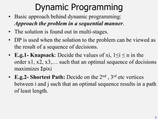
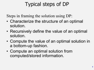
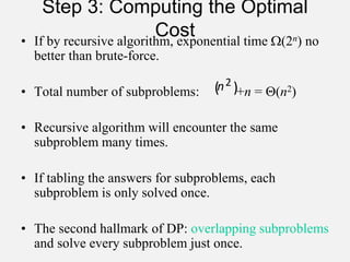
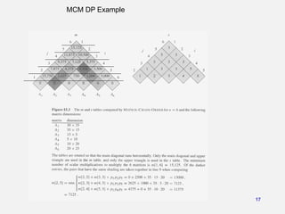
The document discusses various algorithms that use dynamic programming. It begins by defining dynamic programming as an approach that breaks problems down into optimal subproblems. It provides examples like knapsack and shortest path problems. It describes the characteristics of problems solved with dynamic programming as having optimal subproblems and overlapping subproblems. The document then discusses specific dynamic programming algorithms like matrix chain multiplication, string editing, longest common subsequence, shortest paths (Bellman-Ford and Floyd-Warshall). It provides explanations, recurrence relations, pseudocode and examples for these algorithms.

1. Irfan Khatik Analysis of Algorithms and Computing: Chapter 3 1
Analysis of Algorithm and
Computing
Advanced Strategies

2. 2
Dynamic Programming

3. Dynamic Programming
• Basic approach behind dynamic programming:
Approach the problem in a sequential manner.
• The solution is found out in multi-stages.
• DP is used when the solution to the problem can be viewed as
the result of a sequence of decisions.
• E.g.1- Knapsack: Decide the values of xi, 1≤i ≤ n in the
order x1, x2, x3,… such that an optimal sequence of decisions
maximizes Σpixi
• E.g.2- Shortest Path: Decide on the 2nd , 3rd etc vertices
between i and j such that an optimal sequence results in a path
of least length.
3

4. • Dynamic programming is a method for
efficiently solving problems that at first seems to
require a lot of time (possibly exponential), provided we
have:
• Subproblem optimality: the global optimum value can be
defined in terms of optimal subproblems
• Subproblem overlap: the subproblems are not independent,
but instead they overlap (hence, should be constructed bottom-
up).
4
Dynamic Programming

5. Optimal Substructure
• A problem is said to have optimal sub-structure
if the globally optimal solution can be
constructed from locally optimal solutions to
sub problems.
• If it is not possible to make a stepwise optimal
decisions then one approach is to find all
possible decision sequences and find the best
one. This is called Brute Force.
• DP drastically reduces the no. of operations by
avoiding decision sequences that cannot be
optimal.

6. Principle of Optimality
Bellman (1957) stated the principle of optimality
which explains the process of suboptimality as:
• “An optimal policy (or a set of decisions) has
the property that whatever the initial state
and initial decision are, the remaining
decisions must constitute an optimal decision
sequence with regard to the state resulting
from the first decision.”

7. How is it Different from Others?
• Divide and Conquer: the sub-problems are
over-lapping unlike the ones solved using
Divide and Conquer that need to be
independent.
• Greedy Method: In DP, multiple decision
sequences are generated in contrast to GM
where only one decision sequence is
generated.

8. 8
Typical steps of DP
Steps in framing the solution using DP:
• Characterize the structure of an optimal
solution.
• Recursively define the value of an optimal
solution.
• Compute the value of an optimal solution in
a bottom-up fashion.
• Compute an optimal solution from
computed/stored information.

9. Matrix Chain Multiplication
• Problem: given A1, A2, …,An, compute the
product: A1A2…An , find the fastest way (i.e.,
minimum number of multiplications) to compute
it.
• Suppose two matrices A(p,q) and B(q,r), compute
their product C(p,r) in p  q  r multiplications.
• Matrix Multiplication is associative, so the
multiplication A1xA2xA3xA4 can be done in
several different orders.
– For example, M1M2M3 can be calculated as (M1M2)M3
or M1(M2M3).
– The order of multiplication, i.e. the placement of
parenthesis, will determine the number of scalar
multiplications.

10. 10
Matrix-chain multiplication –MCM DP
Intuitive brute-force solution:
• Counting the number of parenthesizations by
exhaustively checking all possible
parenthesizations.
• Let P(n) denote the number of alternative
parenthesizations of a sequence of n matrices:
• P(n) = 1 if n=1
k=1
n-1 P(k)P(n-k) if n2
• The solution to the recursion is (2n).
• So brute-force will not work.

11. 11
MCP DP Steps
• Step 1: structure of an optimal parenthesization
• Let Ai..j (ij) denote the matrix resulting from
AiAi+1…Aj
• Any parenthesization of AiAi+1…Aj must split the
product between Ak and Ak+1 for some k, (ik<j). The
cost = cost of computing Ai..k + cost of computing Ak+1..j
+ # Ai..k  Ak+1..j.
• If k is the position for an optimal parenthesization, the
parenthesization of “prefix” subchain AiAi+1…Ak
within this optimal parenthesization of AiAi+1…Aj
must be an optimal parenthesization.
• AiAi+1…Ak  Ak+1…Aj

12. 12
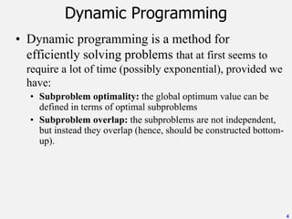
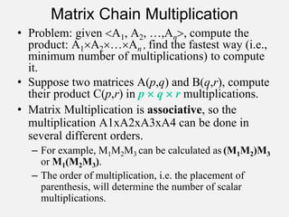
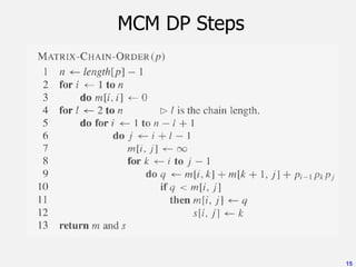
MCP DP Steps
• Step 2: a recursive relation
• Let m[i,j] be the minimum number of
multiplications for AiAi+1…Aj
• m[1,n] will be the answer
If the final multiplication for Aij is Aij= AikAk+1,j
then
• m[i,j] = 0 if i = j
min {m[i,k] + m[k+1,j] +pi-1pkpj } if i<j
ik<j

13. Step 3: Computing the Optimal
Cost
• If by recursive algorithm, exponential time (2n) no
better than brute-force.
• Total number of subproblems: +n = (n2)
• Recursive algorithm will encounter the same
subproblem many times.
• If tabling the answers for subproblems, each
subproblem is only solved once.
• The second hallmark of DP: overlapping subproblems
and solve every subproblem just once.
( )
2
n

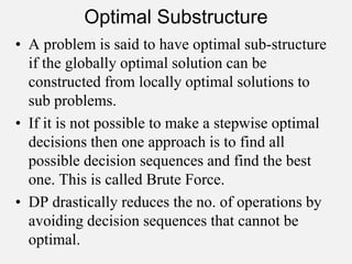
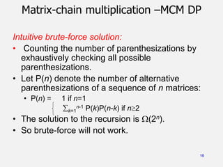
14. Step 3: Algorithm
• Array m[1..n,1..n], with m[i,j] records the
optimal cost for AiAi+1…Aj .
• Array s[1..n,1..n], s[i,j] records index k
which achieved the optimal cost when
computing m[i,j].
• Suppose the input to the algorithm is p=<
p0 , p1 ,…, pn >.

15. 15
MCM DP Steps

16. 16
MCM DP—order of matrix computations
m(1,1) m(1,2) m(1,3) m(1,4) m(1,5) m(1,6)
m(2,2) m(2,3) m(2,4) m(2,5) m(2,6)
m(3,3) m(3,4) m(3,5) m(3,6)
m(4,4) m(4,5) m(4,6)
m(5,5) m(5,6)
m(6,6)

17. 17
MCM DP Example

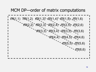
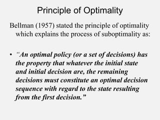
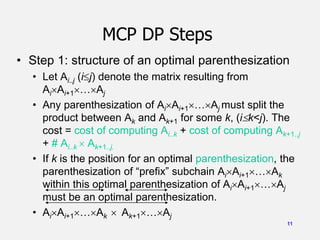
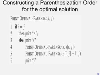
18. MCM DP Steps
• Step 4, constructing a parenthesization
order for the optimal solution.
• Since s[1..n,1..n] is computed, and s[i,j] is
the split position for AiAi+1…Aj , i.e, Ai…As[i,j]
and As[i,j] +1…Aj , thus, the parenthesization
order can be obtained from s[1..n,1..n]
recursively, beginning from s[1,n].

19. Constructing a Parenthesization Order
for the optimal solution
19

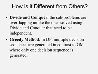
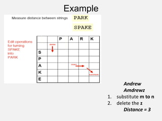
20. String Editing
• Two string are given: X= x₁, x₂, x₃,…,xn and
Y=y₁, y₂, …, ym.
– xi, 1<i<n and yj, 1<j<m are members of Alphabet, a
finite set of symbols.
• Transform X into Y using a sequence of edit
operations on X.
• Set of Edit operations available: Insert[I(xi)],
Delete[D(xi)] and Change[C(xi, yj)].
• Cost associated with each operation.
• Total cost of the sequence of operations is the
sum of cost of each edit operation in sequence.
• Problem: Identify a minimum-cost edit sequence
that transforms X into Y.

21. Example
Andrew
Amdrewz
1. substitute m to n
2. delete the z
Distance = 3

22. • The problem holds Principle of Optimality.
• Define cost(i, j) to be the minimum cost edit
sequence for transforming x₁ to xi to y₁ to yj
for all values of i and j.
• The cost(n,m) is the cost of an optimal edit
sequence.

23. • The recurrence equation for cost(i,j):
• Cost(i, j) = { 0 i=j=0
Cost(i-1, 0) + D(xi) j=0, i>0
Cost(0, j-1) + I(yj) i=0, j>1
Cost’(i, j) i>0, j>0
• Where cost(i,j) =min{ cost(i-1,j) +D(xi),
cost(i-1, j-1) + C(xi, yj), cost(I, j-1) +I(yj)

24. 24
Longest Common Subsequence (LCS)
• DNA analysis, two DNA string comparison.
• DNA string: a sequence of symbols A,C,G,T.
• S=ACCGGTCGAGCTTCGAAT
• Subsequence (of X): is X with some symbols left out.
• Z=CGTC is a subsequence of X=ACGCTAC.
• Common subsequence Z (of X and Y): a subsequence of X and also
a subsequence of Y.
• Z=CGA is a common subsequence of both X=ACGCTAC and
Y=CTGACA.
• Longest Common Subsequence (LCS): the longest one of common
subsequences.
• Z' =CGCA is the LCS of the above X and Y.
• LCS problem: given X=<x1, x2,…, xm> and Y=<y1, y2,…, yn>, find
their LCS.

25. 25
LCS DP –step 1: Optimal Substructure
• Characterize optimal substructure of LCS.
• Theorem 15.1: Let X=<x1, x2,…, xm> (= Xm)
and Y=<y1, y2,…,yn> (= Yn) and Z=<z1, z2,…,
zk> (= Zk) be any LCS of X and Y,
• 1. if xm= yn, then zk= xm= yn, and Zk-1 is the LCS of
Xm-1 and Yn-1.
• 2. if xm yn, then zk  xm implies Z is the LCS of
Xm-1 and Yn.
• 3. if xm yn, then zk  yn implies Z is the LCS of Xm
and Yn-1.

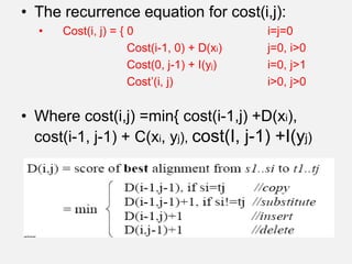
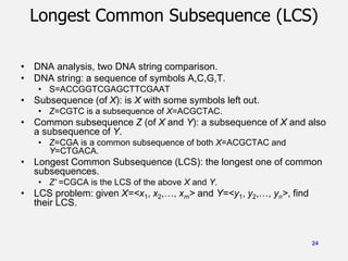
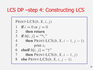
26. 26
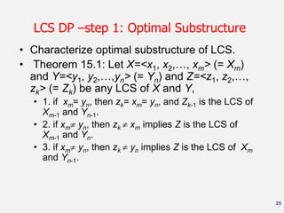
LCS DP –step 2:Recursive Solution
• What the theorem says:
• If xm= yn, find LCS of Xm-1 and Yn-1, then append xm.
• If xm  yn, find LCS of Xm-1 and Yn and LCS of Xm and Yn-
1, take which one is longer.
• Overlapping substructure:
• Both LCS of Xm-1 and Yn and LCS of Xm and Yn-1 will
need to solve LCS of Xm-1 and Yn-1.
• c[i,j] is the length of LCS of Xi and Yj .

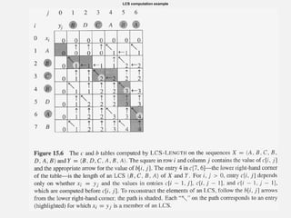
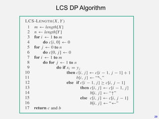
27. 27
LCS DP-- step 3:Computing the Length of LCS
• c[0..m,0..n], where c[i,j] is defined as
above.
• c[m,n] is the answer (length of LCS).
• b[1..m,1..n], where b[i,j] points to the
table entry corresponding to the optimal
subproblem solution chosen when
computing c[i,j].
• From b[m,n] backward to find the LCS.

28. 28
LCS computation example

29. 29
LCS DP Algorithm

30. 30
LCS DP –step 4: Constructing LCS

31. Example: Shortest Path Problem
10
5
3
Goal
Start

32. 25
28
40
Example: Shortest Path Problem
10
5
3
Start Goal

33. 25
28
40
Example: Shortest Path Problem
10
5
3
Start Goal

34. Recall  Greedy Method for
Shortest Paths on a Multi-stage Graph
• Problem
• Find a shortest path from v0 to v3
Is the greedy solution optimal?

35. Recall  Greedy Method for
Shortest Paths on a Multi-stage Graph
• Problem
• Find a shortest path from v0 to v3
Is the greedy solution optimal?
The optimal path


36. Example  Dynamic Programming
min 1,1 3
min 1,2 3
min 0 3
min 1,3 3
min 1,4 3
( , )
( , )
3
1
min
5
7
( , )
( , )
( , )
d v v
d v v
d v v
d v v
d v v

 
 

 
  

 
 

 

37. Dijikstra’s Shortest Path Algorithm
DIJKSTRA (G, w, s)
{
INITIALIZE SINGLE-SOURCE (G, s)
S ← { } // S will ultimately contains vertices of final
shortest-path weights from s
Initialize priority queue Q i.e., Q ← V[G]
while priority queue Q is not empty do
u ← MIN(Q) // Pull out new vertex
S ← S + {u}
// Perform relaxation for each vertex v adjacent to u
for each vertex v in Adj[u] do
Relax (u, v, w)
}
37

38. Irfan Khatik Design and Analysis of Algorithm : Chapter 5 38

39. BellMan-Ford Shortest Path Algorithm
• Detects negative weight cycle
• If no negative weight cycle in graph ,the it
calculates shortest path otherwise return
failure
39

40. Example
z u v x y
1 2 3 4 5

41. z u v x y
1 2 3 4 5
0 0    
1 0 6  7 
Example

42. Example
z u v x y
1 2 3 4 5
0 0    
1 0 6  7 
2 0 6 4 7 2

43. Example
z u v x y
1 2 3 4 5
0 0    
1 0 6  7 
2 0 6 4 7 2
3 0 2 4 7 2

44. Example
z u v x y
1 2 3 4 5
0 0    
1 0 6  7 
2 0 6 4 7 2
3 0 2 4 7 2
4 0 2 4 7 -2

45. Conclusion
• I f Bellman-Ford has not converged after V (G)-
1 iterations, then there cannot be a shortest path
tree, so there must be a negative weight cycle.
• Complexity is O(n³) if Adjacency matrices are
used and O(ne) if lists are used.

46. The All-Pairs Shortest Path Problem:
Floyd-Marshall Algorithm
• Input: A weighted graph, represented by its
weight matrix W.
• Problem: Find the distance between every pair of
nodes.
• Dynamic programming Design:
– Notation: A(k)(i,j) = length of the shortest path from
node i to node j where the label of every intermediary
node is <= k.
• A(0)(i,j) = W[i,j].

47. • Principle of Optimality: We already saw that
any sub-path of a shortest path is a shortest path
between its end nodes.
• Recurrence relation:
• Divide the paths from i to j where every
intermediary node is of label <=k into two groups:
– Those paths that do go through node k
– Those paths that do not go through node k.
• The shortest path in the first group is the shortest
path from i to j where the label of every
intermediary node is <= k-1.
• The length of the shortest path of group 1 is
A(k-1)(i,j)

48. • The length of the shortest path in group 2 is
A(k-1)(i,k) + A(k-1)(k,j)

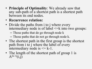
49. • The shortest path in the two groups is the
shorter of the shortest paths of the two groups,
we get
• The algorithm follows:
A(k)(i,j)=min(A(k-1)(i,j), A(k-1)(i,k) + A(k-1)(k,j))
Algorithm AllPaths(cost, a, n)
{
for i=1 to n do
for j=1 to n do
A(0)(i,j) := cost[i,j];
for k=1 to n do
for i=1 to n do
for j=1 to n do
A(k)(i,j)=min(A(k-1)(i,j),A(k-1)(i,k) + A(k-1)(k,j))
}

50. 0/1 Knapsack Problem Merge & Purge

51. 0/1 Knapsack Problem Merge & Purge
Є

52. Σ
Σ
0/1 Knapsack Problem Merge & Purge

53. 0/1 Knapsack Problem Merge & Purge

54. 0/1 Knapsack Problem Merge & Purge

55. 0/1 Knapsack Problem Merge & Purge
Є

56. Informal Knapsack Algorithm

57. Informal Knapsack Algorithm

58. Detailed Knapsack Algorithm

59. Example

60. Travelling Salesman Problem

61. Travelling Salesman Problem

62. Travelling Salesman Problem

63. TSP and Principle of Optimality

64. TSP and Principle of Optimality

65. TSP and Principle of Optimality

66. Complexity
• Complexity of TSP = Θ(n²2ⁿ)
• Since computation of g(I,S) with |S|=k requires
k-1 comparisons.
• Better than solving all n! different tours to find
the best one.
• Space Complexity = O(n2ⁿ)