Download to read offline


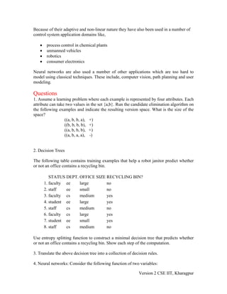
![A B Desired Output
0 0 1
1 0 0
0 1 0
1 1 1
Prove that this function cannot be learned by a single perceptron that uses the step
function as its activation function.
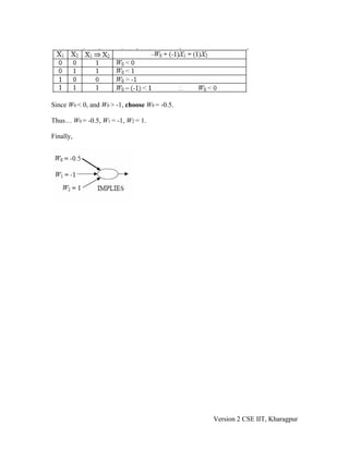
4. Construct by hand a perceptron that can calculate the logic function implies (=>).
Assume that 1 = true and 0 = false for all inputs and outputs.
Solution
1. The general and specific boundaries of the version space are as follows:
S: {(?,b,b,?)}
G: {(?,?,b,?)}
The size of the version space is 2.
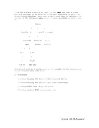
2. The solution steps are as follows:
1. Selecting the attribute for the root node:
YES NO
Status:
Faculty: (3/8)*[ -(2/3)*log_2(2/3) - (1/3)*log_2(1/3)]
Staff: + (3/8)*[ -(0/3)*log_2(0/3) - (3/3)*log_2(3/3)]
Student: + (2/8)*[ -(2/2)*log_2(2/2) - (0/2)*log_2(0/2)]
TOTAL: = 0.35 + 0 + 0 = 0.35
Size:
Large: (3/8)*[ -(2/3)*log_2(2/3) - (1/3)*log_2(1/3)]
Medium: + (3/8)*[ -(1/3)*log_2(1/3) - (2/3)*log_2(2/3)]
Small: + (2/8)*[ -(1/2)*log_2(1/2) - (1/2)*log_2(1/2)]
TOTAL: = 0.35 + 0.35 + 2/8 = 0.95
Version 2 CSE IIT, Kharagpur](https://image.slidesharecdn.com/lesson39-111110110334-phpapp02/85/Lesson-39-8-320.jpg)
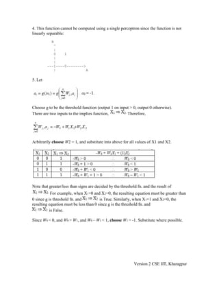
![Dept:
ee: (4/8)*[ -(2/4)*log_2(2/4) - (2/4)*log_2(2/4)]
cs: + (4/8)*[ -(2/4)*log_2(2/4) - (2/4)*log_2(2/4)]
TOTAL: = 0.5 + 0.5 = 1
Since status is the attribute with the lowest entropy, it is selected
as the root node:
Status
/ |
Faculty / | staff student
/ |
1-,3+,6+ 2-,5-,8- 4+,7+
BIN=? BIN=NO BIN=YES
Only the branch corresponding to Status=Faculty needs further
processing.
Selecting the attribute to split the branch Status=Faculty:
YES NO
Dept:
ee: (1/3)*[ -(0/1)*log_2(0/1) - (1/1)*log_2(1/1)]
cs: + (2/3)*[ -(2/2)*log_2(2/2) - (0/2)*log_2(0/2)]
TOTAL: = 0 + 0 = 0
Version 2 CSE IIT, Kharagpur](https://image.slidesharecdn.com/lesson39-111110110334-phpapp02/85/Lesson-39-9-320.jpg)

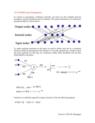
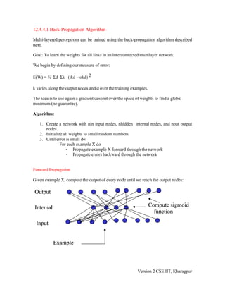
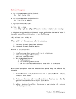
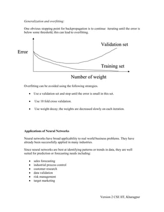
The document discusses multi-layer perceptrons (MLPs) and the backpropagation algorithm. [1] MLPs can learn nonlinear decision boundaries using multiple layers of nodes and nonlinear activation functions. [2] The backpropagation algorithm is used to train MLPs by calculating error terms that are propagated backward to adjust weights throughout the network. [3] Backpropagation finds a local minimum of the error function through gradient descent and may get stuck but works well in practice.