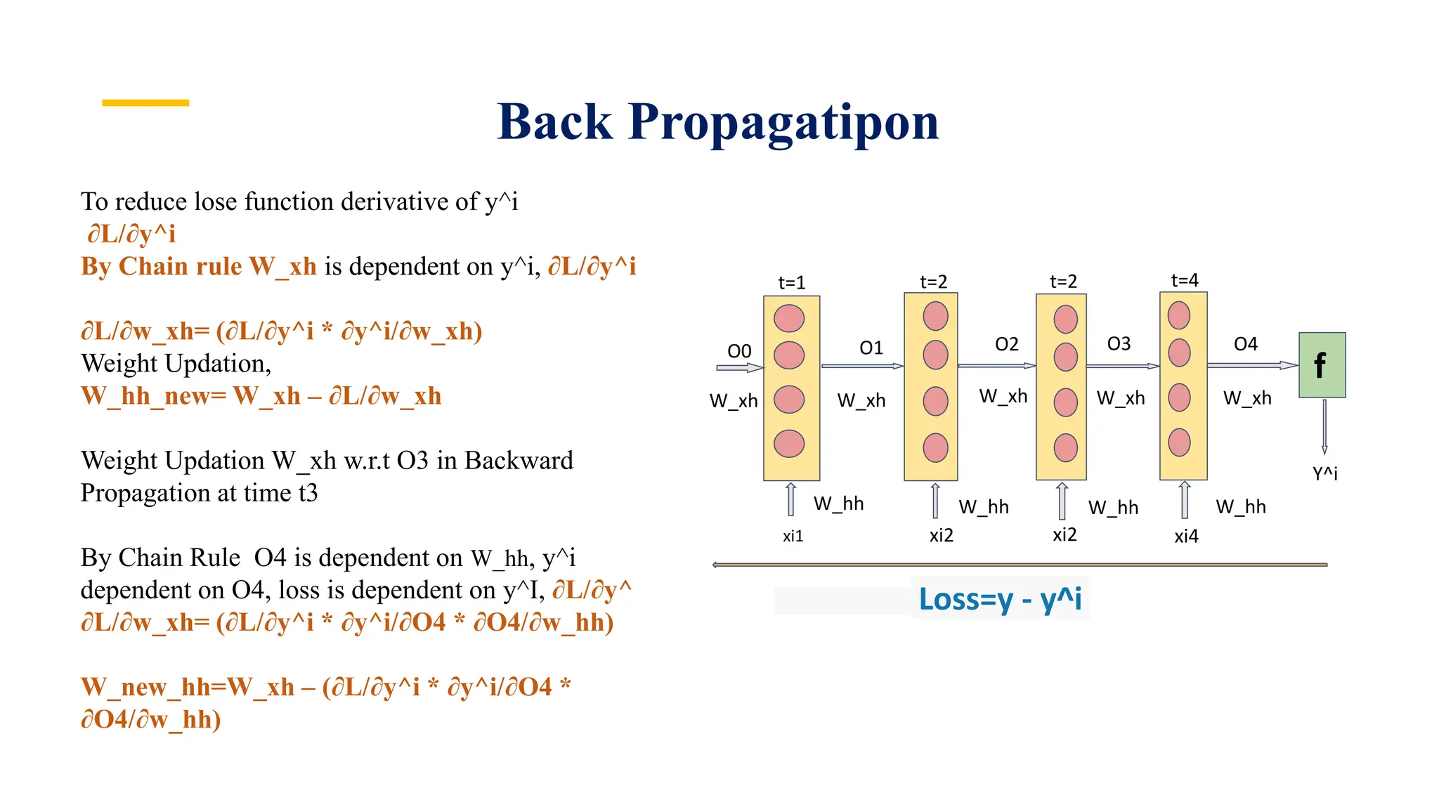
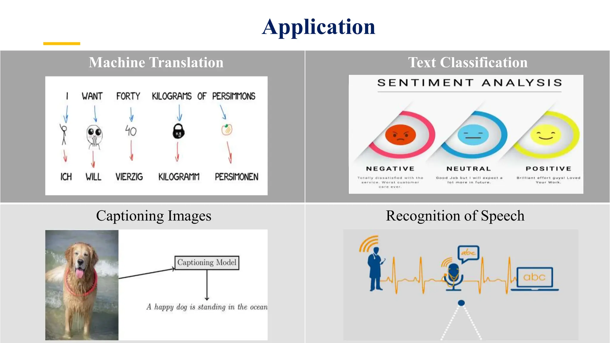
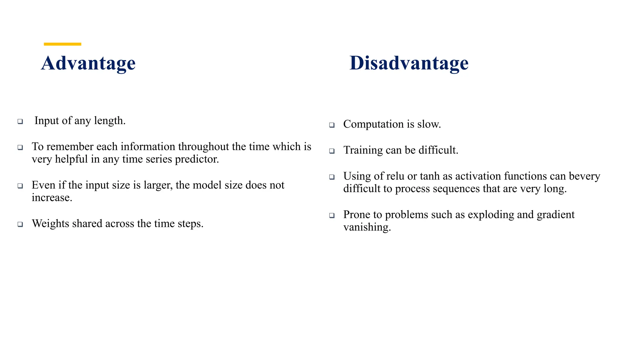
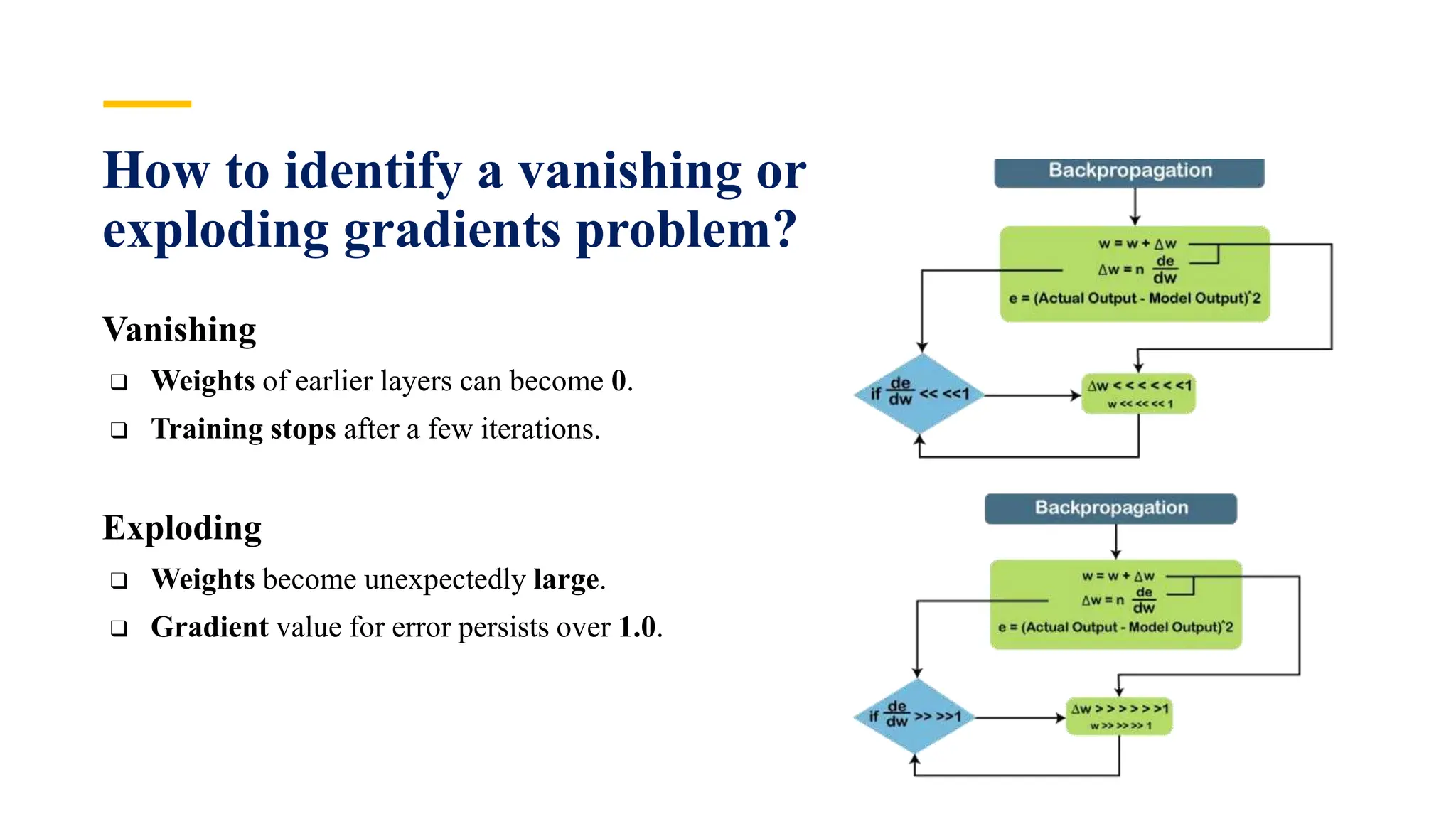
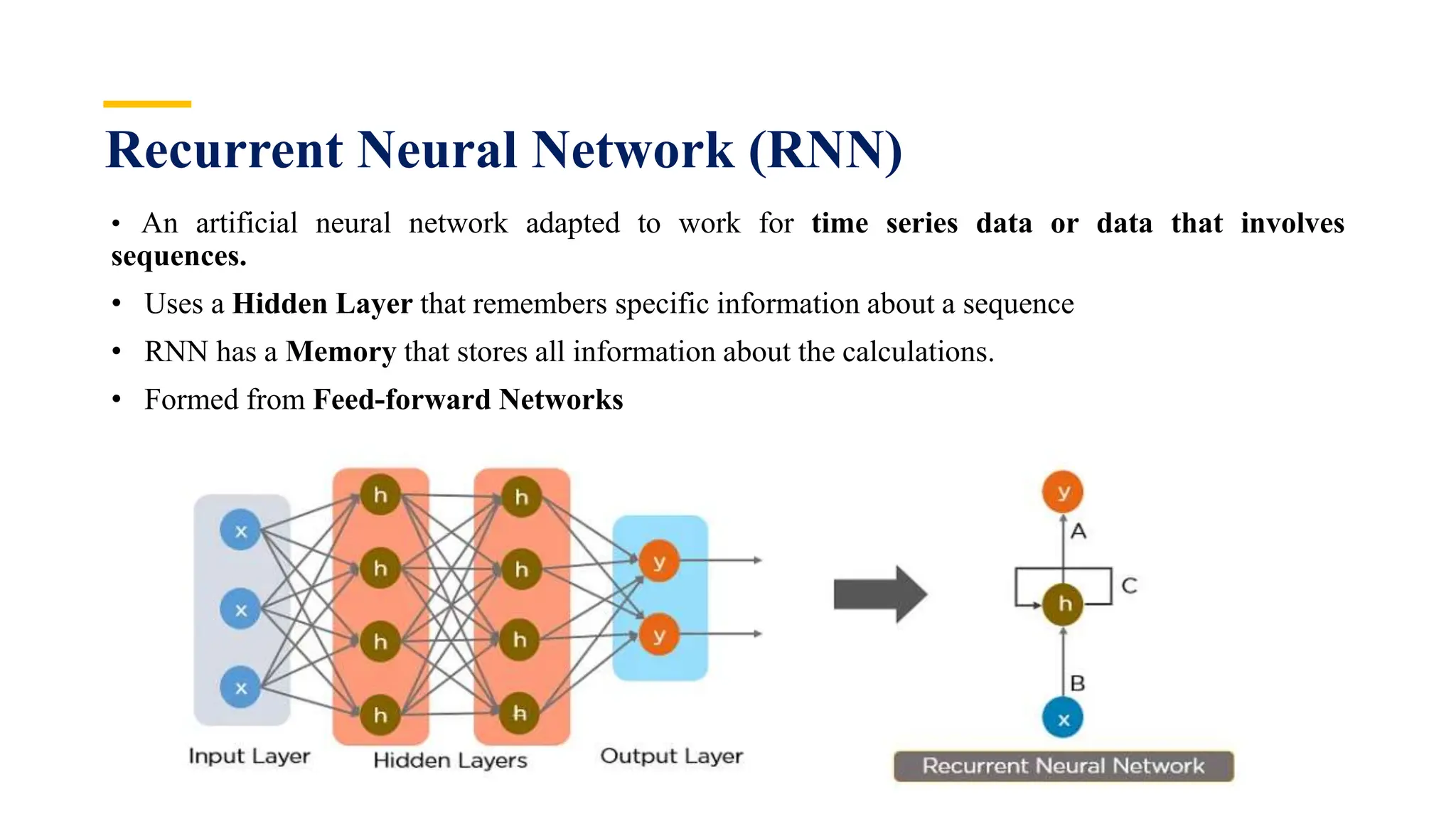
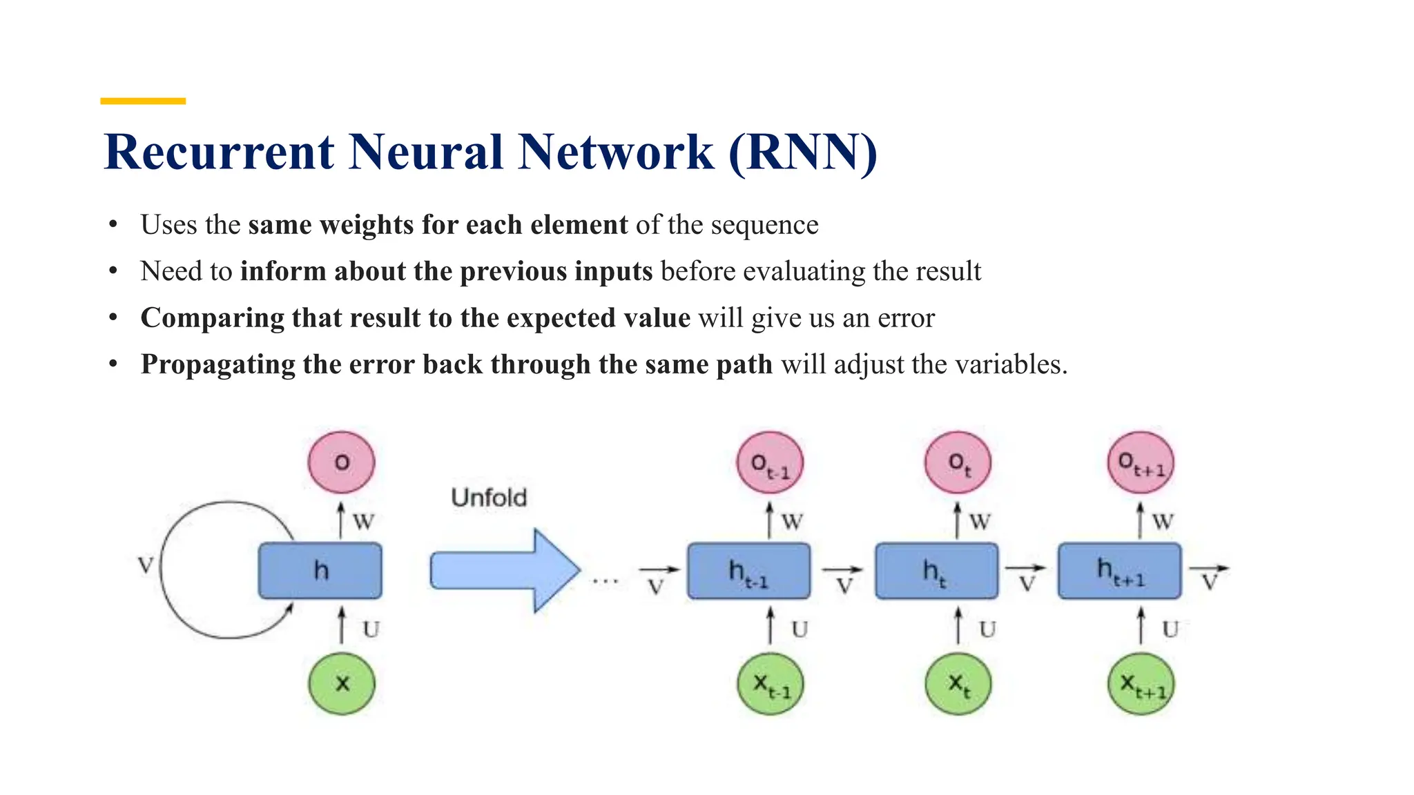
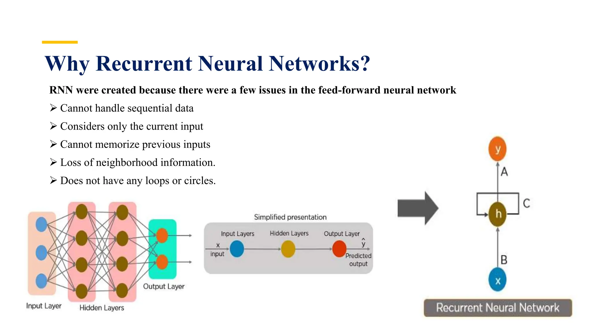
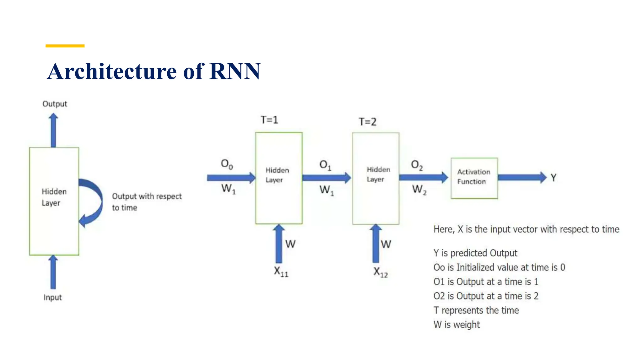
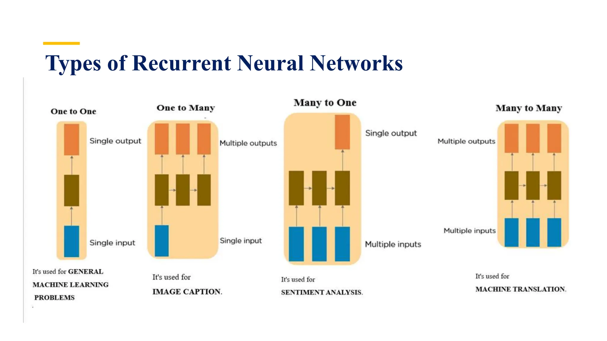
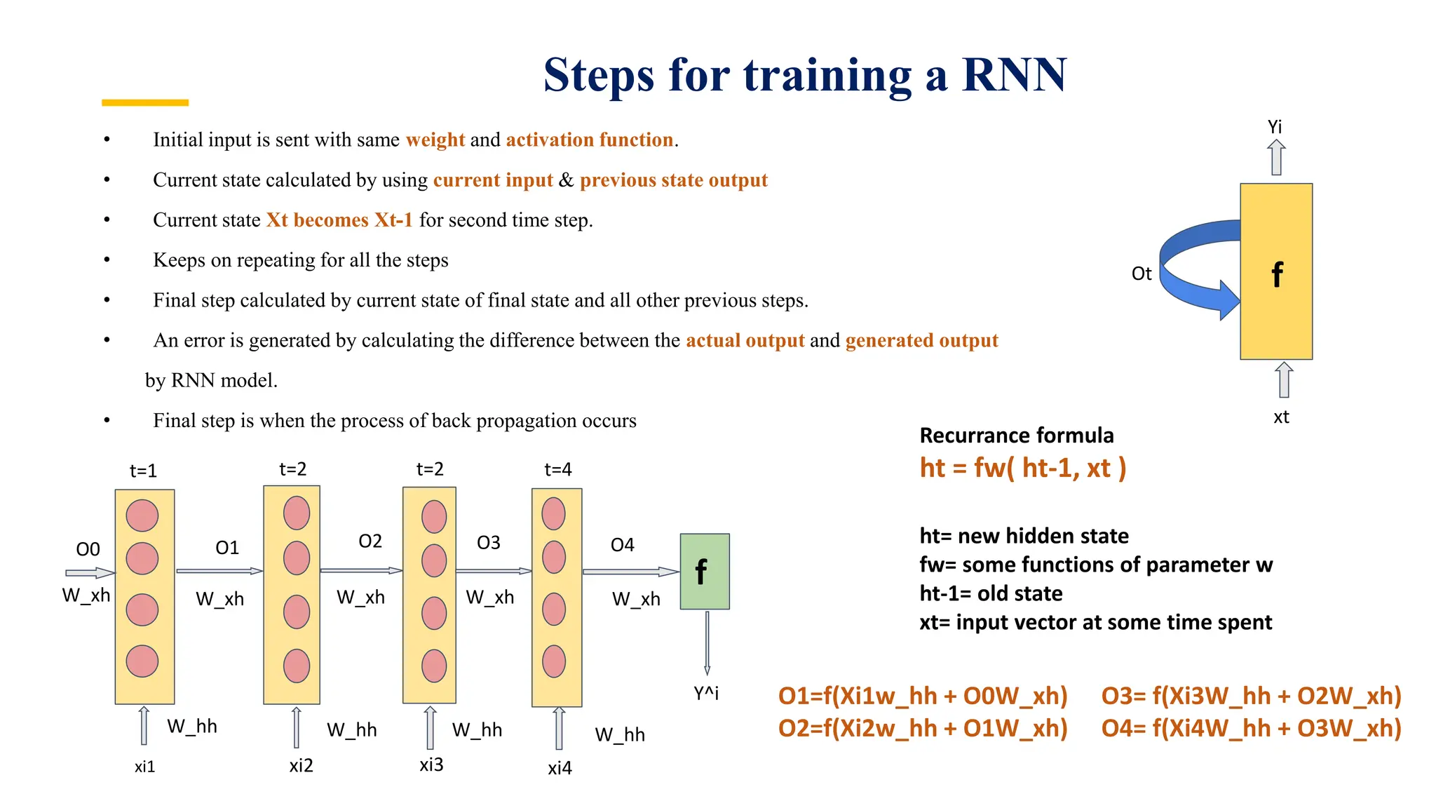
Recurrent Neural Networks (RNNs) are specialized artificial neural networks designed to process sequential or time series data, utilizing a hidden layer to retain information about past inputs. They overcome limitations of feed-forward networks by allowing for memory of previous inputs, adjusting weights through error propagation, and can be trained using backpropagation. Despite their advantages in handling sequences of varying lengths, RNNs face challenges such as vanishing and exploding gradients, which can complicate training and computation.

2. Recurrent Neural Network (RNN)
• An artificial neural network adapted to work for time series data or data that involves
sequences.
• Uses a Hidden Layer that remembers specific information about a sequence
• RNN has a Memory that stores all information about the calculations.
• Formed from Feed-forward Networks

3. Recurrent Neural Network (RNN)
• Uses the same weights for each element of the sequence
• Need to inform about the previous inputs before evaluating the result
• Comparing that result to the expected value will give us an error
• Propagating the error back through the same path will adjust the variables.

4. Why Recurrent Neural Networks?
RNN were created because there were a few issues in the feed-forward neural network
 Cannot handle sequential data
 Considers only the current input
 Cannot memorize previous inputs
 Loss of neighborhood information.
 Does not have any loops or circles.

5. Architecture of RNN

6. Types of Recurrent Neural Networks

7. Steps for training a RNN
• Initial input is sent with same weight and activation function.
• Current state calculated by using current input & previous state output
• Current state Xt becomes Xt-1 for second time step.
• Keeps on repeating for all the steps
• Final step calculated by current state of final state and all other previous steps.
• An error is generated by calculating the difference between the actual output and generated output
by RNN model.
• Final step is when the process of back propagation occurs
xi1
O1
t=1
W_hh
xi2
O2
t=2
xi3
O3
t=2
O0
W_xh
W_hh W_hh W_hh
W_xh W_xh W_xh W_xh
f
Y^i
xi4
O4
t=4
f
Ot
xt
Yi
O1=f(Xi1w_hh + O0W_xh) O3= f(Xi3W_hh + O2W_xh)
O2=f(Xi2w_hh + O1W_xh) O4= f(Xi4W_hh + O3W_xh)
Recurrance formula
ht = fw( ht-1, xt )
ht= new hidden state
fw= some functions of parameter w
ht-1= old state
xt= input vector at some time spent

8. Example: Character-level Language Model
Vocabulary: [h,e,l,o]
Example training sequence: “hello”

9. Continued…
Vocabulary: [h,e,l,o]
At test-time sample characters
one at a time,
feed back to model

10. Back Propagatipon
To reduce lose function derivative of y^i
∂L/∂y^i
By Chain rule W_xh is dependent on y^i, ∂L/∂y^i
∂L/∂w_xh= (∂L/∂y^i * ∂y^i/∂w_xh)
Weight Updation,
W_hh_new= W_xh – ∂L/∂w_xh
Weight Updation W_xh w.r.t O3 in Backward
Propagation at time t3
By Chain Rule O4 is dependent on W_hh, y^i
dependent on O4, loss is dependent on y^I, ∂L/∂y^
∂L/∂w_xh= (∂L/∂y^i * ∂y^i/∂O4 * ∂O4/∂w_hh)
W_new_hh=W_xh – (∂L/∂y^i * ∂y^i/∂O4 *
∂O4/∂w_hh)
Loss=y - y^i
xi1
O1
t=1
W_hh
xi2
O2
t=2
xi2
O3
t=2
f
Y^i
xi4
O4
t=4
O0
W_xh W_xh W_xh W_xh W_xh
W_hh W_hh W_hh

11. Application
Machine Translation Text Classification
Captioning Images Recognition of Speech

12. Advantage
 Computation is slow.
 Training can be difficult.
 Using of relu or tanh as activation functions can bevery
difficult to process sequences that are very long.
 Prone to problems such as exploding and gradient
vanishing.
 Input of any length.
 To remember each information throughout the time which is
very helpful in any time series predictor.
 Even if the input size is larger, the model size does not
increase.
 Weights shared across the time steps.
Disadvantage

13. Vanishing & Exploding
Gradient

14. How to identify a vanishing or
exploding gradients problem?
Vanishing
❑ Weights of earlier layers can become 0.
❑ Training stops after a few iterations.
Exploding
❑ Weights become unexpectedly large.
❑ Gradient value for error persists over 1.0.

15. LSTM

16. Working Process of LSTM
Forget Gate
 Xt: Input to the current timestamp
 Uf: Weight associated with the input
 Ht-1: The Hidden state of the previous timestamp
 Wf: It is the weight matrix associated with the hidden
state

17. Continued
“Bob knows swimming. He told me over the phone
that he had served the navy for four long years.”
Bob single-handedly fought the enemy and died for
his country. For his contributions, brave______.”

18. Continued…

19. Gradient Clipping
Clipping – by – value
A minimum clip value and a maximum clip value.
 g ← ∂C/∂W
• ‖g‖ ≥ max_threshold or ‖g‖ ≤ min_threshold
• g ← threshold (accordingly)
Clipping – by – norm
Clip the gradients by multiplying the unit vector of the
gradients with the threshold.
 g ← ∂C/∂W
 if ‖g‖ ≥ threshold then
 g ← threshold * g/‖g‖

20. Thank You