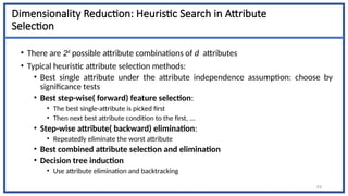
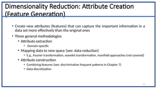
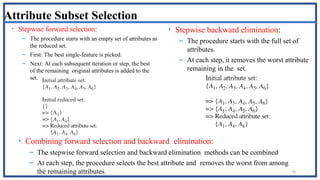
Unit _2 Data Processing.pptx FOR THE DATA SCIENCE STUDENTSHE

1
Data Science
UNIT-2
Data Preprocessing
I-Data Cleaning,
II-Data Integration,
III-Data Reduction,
III-Data Transformation and Data Discretization,

Data Quality: Why Preprocess the Data?
• There are many factors/measures comprising data quality
• Measures for data quality: A multidimensional view
• Accuracy: correct or wrong, accurate or not, errors from instruments , data transmission errors
• Completeness: not recorded, unavailable, user interested attributes may not be available
causing unfilled data
• Consistency: some modified but some not, dangling, …
• Timeliness: timely update? Several sales representatives, however, fail to submit their sales
records on time at the end of the month.
• For a period of time following each month, the data stored in the database are incomplete.
• However, once all of the data are received, it is correct.
• Believability: how trustable the data are correct?
• Interpretability: how easily the data can be understood?
• Suppose that a database, at one point, had several errors, all of which have since been
corrected.
• The data also use many accounting codes, which the sales department does not know how
to interpret. Even though the database is 3

4
Data Mining as Knowledge Discovery
•Data cleaning - to remove noise or
irrelevant data
•Data integration - where multiple data
sources may be combined
•Data selection- where data relevant to the
analysis task are retrieved from the database
•Data transformation -where data are
transformed or consolidated into forms
appropriate for mining by
•performing summary or aggregation
operations
•Data mining - an essential process where
intelligent methods are applied in order to
extract data patterns
•Pattern evaluation to identify the truly
interesting patterns representing knowledge
based
•Knowledge presentation -where
visualization and knowledge representation
techniques are used to present

Major Tasks/Steps in Data Preprocessing
• Data cleaning
• Fill in missing values, smooth noisy data,
• identify or remove outliers, and resolve inconsistencies
• Data integration
• Integration of multiple databases, data cubes, or files
• Data reduction
• Dimensionality reduction
• Numerosity reduction
• Data compression
• Data transformation and data discretization
• Normalization
• Concept hierarchy generation
5

I- Data Cleaning: Incomplete (Missing) Data
• Data is not always available
• E.g., many tuples have no recorded value for several
attributes, such as customer income in sales data
• Missing data may be due to
• equipment malfunction
• inconsistent with other recorded data and thus deleted
• data not entered due to misunderstanding
• certain data may not be considered important at the time of
entry
• not register history or changes of the data
• Missing data may need to be inferred
7

Data Cleaning: How to Handle Missing Data?
• Ignore the tuple: usually done when class label is missing (when doing classification)
—not effective when the % of missing values per attribute varies considerably
• Fill in the missing value manually: tedious + infeasible?
• Fill in it automatically with
• a global constant : e.g., “unknown”, a new class?!
• the attribute mean
• the attribute mean for all samples belonging to the same class: smarter
• the most probable value: inference-based such as Bayesian formula or decision
tree, or use regression to fill
8

9
9
Data Cleaning: Noisy Data
• Noise: random error or variance in a measured variable
• Incorrect attribute values may be due to
• faulty data collection instruments
• data entry problems
• data transmission problems
• technology limitation
• inconsistency in naming convention
• Other data problems which require data cleaning
• duplicate records
• incomplete data
• inconsistent data

10
Data Cleaning: How to Handle Noisy Data?
Binning
first sort data and partition into (equal-frequency) bins
then one can smooth by bin means, smooth by bin median,
smooth by bin boundaries, etc.
Regression
smooth by fitting the data into regression functions
Clustering/Outlier
detect and remove outliers
Combined computer and human inspection
detect suspicious values and check by human (e.g., deal with
possible outliers)

Data Cleaning: Handling Noisy Data: Binning
• Binning:
• This method works on sorted data
• The sorted data is divided into equal frequency buckets/bins
• Binning is of three types:
1. smoothing by bin means
• each value in a bin is replaced by the mean value of the bin.
2. smoothing by bin medians
• each bin value is replaced by the bin median.
3. smoothing by bin boundaries
• the minimum and maximum values in a given bin are identified as the bin boundaries.
• Each bin value is then replaced by the closest boundary value.
11
• “Data smoothing is the technique to handle noisy data
• “smooth” out the data to remove the noise
• data smoothing techniques.
• Binning
• Regression
• Outlier analysis

Data Cleaning: Binning methods
• Equal-width (distance) partitioning
• Divides the range into N intervals of equal size: uniform grid
• if A and B are the lowest and highest values of the attribute, the width of intervals
will be: W = (B –A)/N.
• The most straightforward, but outliers may dominate presentation
• Skewed data is not handled well
• Equal-depth (frequency) partitioning
• Divides the range into N intervals, each containing approximately same number of
samples
• Good data scaling
• Managing categorical attributes can be tricky
12

13
Data Cleaning: Binning Example:
• Sorted data for price (in dollars): 4, 8, 15, 21, 21, 24, 25, 28, 34
• Partition into (equal-frequency-length 3) bins:
• Bin1: 4,8,15 (max=15, min=4)
• Bin 2: 21, 21, 24 (max=24, min=21)
• Bin 3: 25, 28, 34 (max=34,min=25)
• Smoothing by bin means:
• Bin1: 9,9,9. (mean of Bin1=4+8+15/3 =9)
• Bin 2: 22, 22, 22 (mean of Bin2=21+21+24/3 =22)
• Bin 3: 29, 29, 29
• Smoothing by bin boundaries:
• Bin 1: 4,4,15. ( 4 is closer to min=4,replace 4 by 4. 8 is closer to min=4
so replace 8 by 4, 15 is closer to max=15,replace 15 by 15)
• Bin 2: 21, 21, 24
• Bin 3: 25, 25, 34
Use |x2-x1| as
closeness measure

14
Data Cleaning: Handling Noisy Data: Regression
• Regression: Data smoothing can also be done by regression, a
technique that conforms data values to a function.
• Linear regression involves finding the “best” line to fit two
attributes (or variables) so that one attribute can be used to predict
the other.
• Y=mX+c
• Multiple linear regression is an extension of linear regression,
where more than two attributes are involved and the data are fit to
a multidimensional surface.
• Y=m1X1+m2X2+c
• Example:
• Using various normal equations of
Stats the best fitted line can be Y=2X.
• Use Y=2X to predict the correct value at X=3
Which is 6 and replace(smooth) 5.6 by 6
X 0 1 2 3 4
Y 0 2 4 5.6 8
Error data

15
Data Cleaning: Handling Noisy Data: Outlier analysis
Outlier analysis: Outliers may be detected by clustering,
• where similar values are organized into groups, or “clusters.”
• Intuitively, values that fall outside of the set of clusters may be considered outliers
• When Y=X and Y=X2 are fitted then the
Points satisfying these two equations
are taken as two clusters and the errored value 0.5
Which is not into any cluster is identified as outlier .
X 0 1 2 3 4
Y=x 0 1 0.5 3 4
Y=x2
0 1 0.5 9 16 Outlier=0.5

Data Cleaning: ETL (Extraction/Transformation/Loading) : RAPID MINER:
• RapidMiner is a data science software platform developed by the company of the same name
that provides an integrated environment for data preparation, machine learning,
deep learning, text mining, and predictive analytics.
• RapidMiner provides data mining and machine learning procedures including:
data loading and transformation (ETL),
• Data pre-processing and visualization, predictive analytics and statistical modelling,
evaluation, and deployment.
• RapidMiner is written in the Java programming language.
• RapidMiner provides a GUI to design and execute analytical workflows.
• Those workflows are called “Processes” in RapidMiner and they consist of multiple
“Operators”.
• Each operator performs a single task within the process, and the output of each operator
forms the input of the next one
• Documentation link: https://docs.rapidminer.com/
16

17
Data Cleaning: Snapshot of rapid miner : ETL
(Extraction/Transformation/Loading)

18
Handle missing values -Cleaning and
Munging
• During cleaning and munging in data science, handling missing values
is one of the most common tasks. The real-life data might contain missing
values which need a fix before the data can be used for analysis. We can
handle missing values by:
1. Either removing the records that have missing values or
2. Filling the missing values using some statistical technique or by
gathering data understanding.
• A rule of thumb is that you can drop the missing values if they make up
for less than five percent of the total number of records but however it
depends on the analysis, the importance of the missing values, the size of
the data, and the use case we are working on.

19
Manipulating Data
• Data Manipulation Meaning: Manipulation of data is the
process of manipulating or changing information to make it
more organized and readable.

20
Hypothesis and Inference
• Statistical Inference
• Using data analysis and statistics to make conclusions
about a population is called statistical inference.
• The main types of statistical inference are:
Estimation
Hypothesis testing
• Hypothesis testing is a method to check if a claim about
a population is true. More precisely, it checks how likely it
is that a hypothesis is true is based on the sample data.

23
Data Integration:
Data integration:
Combines data from multiple sources into a coherent store.
Approaches in Data Integration
1. Entity identification problem:
2. Tuple Duplication:
3. Detecting and resolving data value conflicts
4. Redundancy and Correlation Analysis

1. Entity identification problem
• Schema integration:
Mismatching attribute names
Identify real world entities from multiple data sources,
e.g., Bill Clinton = William Clinton
e.g., A.cust-id  B.cust-#
Integrate metadata from different sources
• Object matching: Mismatching structure of data
Ex: Discount issues
Currency type
24

2. Tuple Duplication:
• The use of denormalized tables is another
source of data redundancy.
Inconsistencies often arise between
various duplicates due to inaccurate data
entry.
25
Name DOB Branch Occupation Address
A 25 HYD Govt TPG
B 30 TH Govt RJY
A 25 HYD Private TPG
D 30 IBP Private RJY

3. Detecting and resolving data value conflicts
For the same real world entity, attribute values from different sources are
different.
Possible reasons:
different representations, Ex: Total sales for month single store/all stores
different scales, e.g., metric vs. British units (e.g., GPA in US and
China)
26

• Redundant data occur often when integration of multiple databases
• Object identification: The same attribute or object may have different
names in different databases
• Derivable data: One attribute may be a “derived” attribute in another
table, e.g., annual revenue
• Redundant attributes may be able to be detected by correlation analysis
• Careful integration of the data from multiple sources may help reduce/avoid
redundancies and inconsistencies and improve mining speed and quality
27

Correlation
Correlation analysis is a method of statistical evaluation used to study the strength of a
relationship between two, numerically measured, continuous variables.
 Computed as Correlation co-efficient
 Value ranges between – (-1) to (+1)
 Positively Correlated, Negatively correlated,
Not correlated
 The strength of a correlation indicates how
strong the relationship is between the two
variables. The strength is determined by the
numerical value of the correlation

34
SUBJECT AGE X
GLUCOSE
LEVEL Y
XY X2
Y2
1 43 99 4257 1849 9801
2 21 65 1365 441 4225
3 25 79 1975 625 6241
4 42 75 3150 1764 5625
5 57 87 4959 3249 7569
6 59 81 4779 3481 6561
Σ 247 486 20485 11409 40022
The correlation coefficient =
6(20,485) – (247 × 486) / [√[[6(11,409) – (2472
)] × [6(40,022) – 4862
]]]. = 0.5298 (strength and direction)
The range of the correlation coefficient is from -1 to 1.
here result is 0.5298 or 52.98%, which means the variables have a moderate positive correlation( some what more ). We
cant infer with 52.98% correlation that age has impact on rise in glucose levels. We need more data to analyze
From our table:
Σx = 247
Σy = 486
Σxy = 20,485
Σx2
= 11,409
Σy2
= 40,022
n is the sample
size=6
Example problem:
Business problem: The healthcare industry want to develop a
medication to control glucose levels. For this it want to study does age
have impact on raise in glucose levels

37
Redundancy and Correlation Analysis: Chi-square Test
• A correlation relationship between two categorical (discrete) attributes, A and B, can
be discovered by a X2 (chi-square) test.

39
Chi-Square Calculation: An Example
• Suppose that a group of 1,500 people was surveyed.
• The observed frequency (or count) of each possible joint
event is summarized in the contingency table shown
• The numbers in parentheses are the expected frequencies
(calculated based on the data distribution for both
attributes using Equation eij).
• Are like_science_fiction and play_chess
correlated?
Play chess Not play chess Sum (row)
Like science fiction 250(90) 200(360) 450
Not like science fiction 50(210) 1000(840) 1050
Sum(col.) 300 1200 1500

40
• For example, the expected frequency for the cell
(play_chess, fiction) is
11
e 
count( play _ chess)* count(like_science_fiction)

300 * 450

90
N
1500
• Notice that
– the sum of the expected frequencies must equal the
total observed frequency for that row, and
– the sum of the expected frequencies in any column
must also equal the total observed frequency for that
column.

41
• We can get X2 by:
• For this 2 x 2 table, the degrees of freedom are (2-1)(2-1) = 1. ((no. of rows-
1)*(no.of columns-1))
• For 1 degree of freedom, the X2 value needed to reject the hypothesis at the
0.001 significance level is 10.828 (taken from the table of upper percentage
points of the X2 distribution, typically available from any textbook on
statistics).
• Since our computed value is above this, we can reject the hypothesis that play
chess and preferred reading are independent and conclude that the two
attributes are (strongly) correlated for the given group of people.

Data Reduction strategies:
• Data reduction: Obtain a reduced representation of the data set that is much smaller
in volume but yet produces the same (or almost the same) analytical results
• Why data reduction? — A database/data warehouse may store terabytes of data.
Complex data analysis may take a very long time to run on the complete data set.
• Data reduction strategies
1.Data cube aggregation
3. Dimensionality reduction-remove unimportant attributes/variables
Eliminate the redundant attributes: which are weekly important across the
data.
• Wavelet transforms/ Data compression
• Principal Components Analysis (PCA)
• Feature subset selection, feature creation
4. Numerosity reduction- replace original data volume by smaller forms of data
• Regression and Log-Linear Models
• Histograms, clustering, sampling
• Data cube aggregation
43

1. Data cube aggregation
44
Year/Quarter 2014 2015 2016 2017 Year Sales
Quarter 1 200 210 320 230 2014 1640
Quarter 2 400 440 480 420 2015 1710
Quarter 3 480 480 540 460 2016 2020
Quarter 4 560 580 680 640 2017 1750
For example, the data consists of AllElectronics sales per quarter for the years 2014 to
2017.You are, however, interested in the annual sales, rather than the total per quarter. Thus,
the data can be aggregatedso that the resulting data summarize the total sales per year instead
of per quarter

45
2. Dimensionality Reduction
• Know about Curse of dimensionality
• When dimensionality increases, data becomes increasingly sparse
• Density and distance between points, which is critical to clustering, outlier analysis,
becomes less meaningful
• The possible combinations of subspaces will grow exponentially
• What is Dimensionality reduction
• Method of eliminating irrelevant features so as to reduce noise
• Is proposed to avoid the curse of dimensionality
• Reduce time and space required in data mining
• Allow easier visualization of data (quite messy to visualize huge data)
• Dimensionality reduction techniques
• Wavelet transforms
• Principal Component Analysis
• Supervised and nonlinear techniques (e.g., feature selection)

46
Dimensionality Reduction: Wavelet Transform
• The discrete wavelet transform (DWT) is a linear signal processing technique that,
when applied to a data vector, transforms it to a numerically different vector, of
wavelet coefficients.
• The two vectors are of the same length. When applying this technique to data
reduction, we consider each tuple as an n-dimensional data vector, that is, X=(x1,x2,
…………,xn), depicting n measurements made on the tuple from n database
attributes .
• For example, all wavelet coefficients larger than some user-specified threshold
can be retained. All other coefficients are set to 0. The resulting data
representation is therefore very sparse, so that can take advantage of data sparsity
are computationally very fast if performed in wavelet space.
• Given a set of coefficients, an approximation of the original data can be
constructed by applying the inverse of the DWT used.

Dimensionality Reduction: Sequence Data and
Wavelet Function
47
A continuous wavelet function
Haar2 Daubechie4

Dimensionality Reduction: Wavelet Transformation
• Discrete wavelet transform (DWT): linear signal processing, multi-resolutional
analysis
• Similar to discrete Fourier transform (DFT), but better lossy compression,
localized in space
• Method:
• Length, L, must be an integer power of 2 (padding with 0’s, when necessary)
• Each transform has 2 functions: sum, difference
• Applies to pairs of data, resulting in two set of data of length L/2
• Applies two functions recursively, until reaches the desired length
• Compressed approximation: store only a small fraction of the strongest of the
wavelet coefficients
48

49
0 1 2 3 4 3 2 1
1 1 -1 -1 1 5 7 3
0 0 2 -2 4 -4 6 10
0 0 -4 0 -8 0 4 16
An example

DWT for Image Compression
Image
Low Pass High Pass
Low Pass High Pass
Low Pass High Pass
50

Dimensionality Reduction: Principal Component Analysis (PCA)
• Given N data vectors from d-dimensions, find k ≤ d orthogonal
vectors (principal components) that can be best used to represent
data
• Steps
• Normalize input data
• Compute k orthonormal (unit) vectors, i.e., principal
components
• The principal components are sorted in order of decreasing
“significance” or strength
• Since the components are sorted, the size of the data can be
reduced by eliminating the weak components, i.e., those with
low variance. (i.e., using the strongest principal components, it
is possible to reconstruct a good approximation of the original
data)
• Used when the number of dimensions is large
51

Dimensionality Reduction: PCA Method
52
1
( )

Dimensionality Reduction: Attribute Subset
Selection
•Attribute subset selection reduces the data set size by removing irrelevant or redundant
attributes (or dimensions). The goal of attribute subset selection is to find a minimum set of
attributes. It reduces the number of attributes appearing in the discovered patterns, helping to
make the patterns easier to understand.
•To find out a ‘good’ subset from the original attributes
• Another way to reduce dimensionality of data
• Redundant attributes
• Duplicate much or all of the information contained in one or more other attributes
• E.g., purchase price of a product and the amount of sales tax paid
• Irrelevant attributes
• Contain no information that is useful for the data mining task at hand
• E.g., students' ID is often irrelevant to the task of predicting students' GPA
53

Dimensionality Reduction: Heuristic Search in Attribute
Selection
• There are 2d
possible attribute combinations of d attributes
• Typical heuristic attribute selection methods:
• Best single attribute under the attribute independence assumption: choose by
significance tests
• Best step-wise( forward) feature selection:
• The best single-attribute is picked first
• Then next best attribute condition to the first, ...
• Step-wise attribute( backward) elimination:
• Repeatedly eliminate the worst attribute
• Best combined attribute selection and elimination
• Decision tree induction
• Use attribute elimination and backtracking
54

55
Heuristic Search in Attribute Selection

56
Dimensionality Reduction: Attribute Creation
(Feature Generation)
• Create new attributes (features) that can capture the important information in a
data set more effectively than the original ones
• Three general methodologies
• Attribute extraction
• Domain-specific
• Mapping data to new space (see: data reduction)
• E.g., Fourier transformation, wavelet transformation, manifold approaches (not covered)
• Attribute construction
• Combining features (see: discriminative frequent patterns in Chapter 7)
• Data discretization

3. Numerosity Reduction
• Reduce data volume by choosing alternative, smaller forms of data
representation
• Parametric methods
• Regression:
Simple linear regression
Multiple linear regression
Assume the data fits some model, estimate model parameters, store
only the parameters, and discard the data (except possible outliers)
• Log-linear models—obtain value at a point in m-D space as the product on
appropriate marginal subspaces
• Non-parametric methods
• Do not assume models
• Major families: Histograms, Clustering, Sampling, Cube aggregation
57

Parametric methods: Regression Analysis
• Regression analysis: A collective name for
techniques for the modeling and analysis of
numerical data consisting of values of a
dependent variable (also called response
variable or measurement) and of one or more
independent variables (aka. explanatory
variables or predictors)
• The parameters are estimated so as to give a
"best fit" of the data
• Most commonly the best fit is evaluated by
using the least squares method, but other
criteria have also been used
• Used for prediction (including
forecasting of time-series data),
inference, hypothesis testing,
and modeling of causal
relationships
58
y
x
y = x + 1
X1
Y1
Y1’

Parametric methods : Regress Analysis and Log-Linear Models
• Linear regression: Y = w X + b
• Two regression coefficients, w and b, specify the line and are to be estimated by using the
data at hand
• Using the least squares criterion to the known values of Y1, Y2, …, X1, X2, ….
• Multiple regression: Y = b0 + b1 X1 + b2 X2
• Many nonlinear functions can be transformed into the above
• Log-linear models:
• Approximate discrete multidimensional probability distributions
• Estimate the probability of each point (tuple) in a multi-dimensional space for a set of
discretized attributes, based on a smaller subset of dimensional combinations
• Useful for dimensionality reduction and data smoothing
59

Nonparametric methods : Histogram Analysis
• Divide data into buckets and store
average (sum) for each bucket
• Partitioning rules:
• Equal-width: equal bucket
range
• Equal-frequency (or equal-
depth)
60
0
5
10
15
20
25
30
35
40
10000 30000 50000 70000 90000

Nonparametric methods : Clustering
• Partition data set into clusters based on similarity, and store cluster representation
(e.g., centroid and diameter) only
• Can be very effective if data is clustered but not if data is “smeared”
• Can have hierarchical clustering and be stored in multi-dimensional index tree
structures
• There are many choices of clustering definitions and clustering algorithms
61

Nonparametric methods : Sampling
• Sampling: obtaining a small sample s to represent the whole data set N
• Allow a mining algorithm to run in complexity that is potentially sub-linear to
the size of the data
• Key principle: Choose a representative subset of the data
• Simple random sampling may have very poor performance in the
presence of skew
• Develop adaptive sampling methods, e.g., stratified sampling:
• Note: Sampling may not reduce database I/Os (page at a time)
62

Nonparametric methods : Types of Sampling
• Simple random sampling
• There is an equal probability of selecting any particular item
• Sampling without replacement
• Once an object is selected, it is removed from the population
• Sampling with replacement
• A selected object is not removed from the population
• Stratified sampling:
• Partition the data set, and draw samples from each partition
(proportionally, i.e., approximately the same percentage of the data)
• Used in conjunction with skewed data
63

64
Nonparametric methods : Sampling: With or without
Replacement
SRSWOR
(simple random
sample without
replacement)
SRSWR
Raw Data

Sampling: Cluster or Stratified Sampling
65
Raw Data Cluster/Stratified Sample

66
Nonparametric methods : Data Cube Aggregation
•Data cube aggregation, where aggregation operations are applied to
the data for construction of a data cube.
•Data cubes store multidimensional aggregated information. Each cell
holds an aggregate data value, corresponding to the data point in
multidimensional space.
•Concept hierarchies may exist for each attribute, allowing the analysis
of data at multiple level of abstraction.
•Data cubes provide fast access to pre computed summarized data,
thereby benefiting on-line analytical processing as well as data mining.

67
Nonparametric methods : Data Cube Aggregation
•The cube can be created in three ways:
 Based cuboid- The cube created at the lowest level of abstraction is referred to as base
cuboid.
 Lattice of cuboids- Data cubes created for varying levels of abstraction are often
referred to as cuboids.
 Apex cuboid - A cube at highest level of abstraction is the apex cuboid

68
IV- Data Transformation
• Data transformation
The data are transformed into forms appropriate for mining.
• Data transformation tasks:
1. Smoothing: Remove the noise from the data. Techniques
includes Binning, Regression, Clustering.
2. Normalization
3. Attribute construction, Subset selection
4. Aggregation
5. Discretization
6. Generalization

69
Data Transformation Tasks
• Normalization
– the attribute data are scaled so as to fall within a
small specified range, such as -1.0 to 1.0, 0.0 to 1.0
• Attribute construction (or feature construction)
– new attributes are constructed and added from the given
set of attributes to help the mining process.
• Aggregation
– summary or aggregation operations are applied to the data.
– For example, the daily sales data may be aggregated so
as to compute monthly and annual total amounts.

70
Data Transformation Tasks
• Discretization
– Dividing the range of a continuous attribute into intervals
– For example, values for numerical attributes, like age, may be mapped
to higher-level concepts, like youth, middle- aged, and senior.
• Generalization
– where low-level or “primitive” (raw) data are replaced by higher-level
concepts through the use of concept hierarchies.
– For example, categorical attributes, like street, can be generalized to
higher-level concepts, like city or country.

71
2. Normalization
• An attribute is normalized by scaling its values so that they fall within a small
specified range, such as 0.0 to 1.0.
• Normalization is particularly useful for classification algorithms involving
– neural networks
– distance measurements such as nearest-neighbor classification and clustering.
• If using the neural network backpropagation algorithm for classification mining,
normalizing the input values for each attribute measured in the training instances will
help speed up the learning phase.
• For distance-based methods, normalization helps prevent attributes with initially large
ranges (e.g., income) from out-weighing attributes with initially smaller ranges (e.g.,
binary attributes).
• Normalization methods
I. Min-max normalization
II. z-score normalization
III. Normalization by decimal scaling

72
Min-max Normalization
• Min-max normalization
– performs a linear transformation on the original data.
• Suppose that:
– minA and maxA are the minimum and maximum values of
an attribute, A.
• Min-max normalization maps a value, v, of A to v′ in
the range [new_minA, new_maxA] by computing:
maxA  minA
v  minA
v'  (new _ maxA  new _ minA)  new _ minA

Normalization
• Min-max normalization: to [new_minA, new_maxA]
• Ex. Let income range $12,000 to $98,000 normalized to [0.0, 1.0]. Then
$73,000 is mapped to
• Z-score normalization (μ: mean, σ: standard deviation):
• Ex. Let μ = 54,000, σ = 16,000. Then
• Normalization by decimal scaling
716
.
0
0
)
0
0
.
1
(
000
,
12
000
,
98
000
,
12
600
,
73





225
.
1
000
,
16
000
,
54
600
,
73


73
A
A
A
A
A
A
min
new
min
new
max
new
min
max
min
v
v _
)
_
_
(
' 




A
A
v
v




'
j
v
v
10
' Where j is the smallest integer such that Max(|ν’|) < 1

74
3. Data Aggregation
• On the left, the sales are shown per quarter. On the right, the data are aggregated to provide the
annual sales
• Sales data for a given branch of AllElectronics for the years 2002 to 2004.
• Data cubes store multidimensional aggregated information.
• Data cubes provide fast access to precomputed, summarized data, thereby benefiting on-line analytical
processing as well as data mining.
• A data cube for sales at AllElectronics.

75
4. Attribute Construction
• Attribute construction (feature construction)
– new attributes are constructed from the given attributes and added in order to help improve
the accuracy and understanding of structure in high-dimensional data.
• Example
– we may wish to add the attribute area based on the attributes height and width.
• By attribute construction can discover missing information.
• Why attribute subset selection
– Data sets for analysis may contain hundreds of attributes, many of which may be irrelevant
to the mining task or redundant.
• For example,
– if the task is to classify customers as to whether or not they are likely to purchase a popular
new CD at AllElectronics when notified of a sale, attributes such as the customer’s
telephone number are likely to be irrelevant, unlike attributes such as age or music_taste.

76
Attribute Subset Selection
• Using domain expert to pick out some of the useful attributes
– Sometimes this can be a difficult and time-consuming task, especially when the behavior of
the data is not well known.
• Leaving out relevant attributes or keeping irrelevant attributes result in discovered
patterns of poor quality.
• In addition, the added volume of irrelevant or redundant attributes can slow
down the mining process.
• Attribute subset selection (feature selection):
– Reduce the data set size by removing irrelevant or redundant attributes
• Goal:
– select a minimum set of features (attributes) such that the probability distribution of different
classes given the values for those features is as close as possible to the original distribution
given the values of all features
– It reduces the number of attributes appearing in the discovered patterns, helping to make the
patterns easier to understand.

77
• How can we find a ‘good’ subset of the original attributes?
– For n attributes, there are 2n possible subsets.
– An exhaustive search for the optimal subset of attributes can be prohibitively expensive, especially as
n increase.
– Heuristic methods that explore a reduced search space are commonly used for attribute subset
selection.
– These methods are typically greedy in that, while searching through attribute space, they always make
what looks to be the best choice at the time.
– Such greedy methods are effective in practice and may come close to estimating an optimal
solution.
• Heuristic methods:
1. Step-wise forward selection
2. Step-wise backward elimination
3. Combining forward selection and backward elimination
4. Decision-tree induction
• The “best” (and “worst”) attributes are typically determined using:
– the tests of statistical significance, which assume that the attributes are independent of one another.
– the information gain measure used in building decision trees for classification.

78
• Stepwise forward selection:
– The procedure starts with an empty set of attributes as
the reduced set.
– First: The best single-feature is picked.
– Next: At each subsequent iteration or step, the best
of the remaining original attributes is added to the
set.
• Stepwise backward elimination:
– The procedure starts with the full set of
attributes.
– At each step, it removes the worst attribute
remaining in the set.
• Combining forward selection and backward elimination:
– The stepwise forward selection and backward elimination methods can be combined
– At each step, the procedure selects the best attribute and removes the worst from among
the remaining attributes.

79
• Decision tree induction:
– Decision tree algorithms, such as ID3, C4.5, and
CART, were originally intended for classification.
– Decision tree induction constructs a flowchart-like
structure where each internal (nonleaf) node denotes a
test on an attribute, each branch corresponds to an
outcome of the test, and each external (leaf) node denotes
a class prediction.
– At each node, the algorithm chooses the “best” attribute
to partition the data into individual classes.
– When decision tree induction is used for attribute
subset selection, a tree is constructed from the given
data.
– All attributes that do not appear in the tree are assumed
to be irrelevant.

80
5. Generalization
• Generalization is the generation of concept hierarchies for categorical data
• Categorical attributes have a finite (but possibly large) number of distinct
values, with no ordering among the values.
• Examples include
– geographic location,
– job category, and
– itemtype.
• A relational database or a dimension location of a data warehouse may contain the
following group of attributes: street, city, province or state, and country.
• A user or expert can easily define a concept hierarchy by specifying ordering of the
attributes at the schema level.
• A hierarchy can be defined by specifying the total ordering among these attributes at the
schema level, such as:
◆ street < city < province or state < country

6. Discretization
• Three types of attributes:
• Nominal — values from an unordered set, e.g., color, profession
• Ordinal — values from an ordered set, e.g., military or academic rank
• Continuous — real numbers, e.g., integer or real numbers
• Discretization:
• Divide the range of a continuous attribute into intervals
• Some classification algorithms only accept categorical attributes.
• Reduce data size by discretization
81

Discretization and Concept Hierarchy
Discretization
• Reduce the number of values for a given continuous attribute by dividing
the range of the attribute into intervals
• Interval labels can then be used to replace actual data values
• Supervised vs. unsupervised
• Split (top-down) vs. merge (bottom-up)
• Discretization can be performed recursively on an attribute
Concept hierarchy formation
• Recursively reduce the data by collecting and replacing low level concepts
(such as numeric values for age) by higher level concepts (such as young,
middle-aged, or senior)
82

Discretization and Concept Hierarchy Generation for
Numeric Data
• Typical methods: All the methods can be applied recursively
• Binning
• Top-down split, unsupervised,
• Histogram analysis
• Top-down split, unsupervised
• Clustering analysis
• Either top-down split or bottom-up merge, unsupervised
• Entropy-based discretization: supervised, top-down split
• Interval merging by 2
Analysis: supervised, bottom-up merge
83

Entropy-Based Discretization
• Entropy is calculated based on class distribution of the samples in the set.
Given m classes, the entropy of S1 is
• where pi is the probability of class i in S1
• Given a set of samples S, if S is partitioned into two intervals S1 and S2 using
boundary T, the information gain after partitioning is
• The boundary that minimizes the entropy function over all possible boundaries
(i.e. maximize information is selected as a binary discretization)
• The process is recursively applied to partitions obtained until some stopping
criterion is met
• Such a boundary may reduce data size and improve classification accuracy 84
1 2
1 2
| | | |
( , ) ( ) ( ( ) ( ))
| | | |
S S
I S T Entropy S Entropy Entropy
S S
S S
  




m
i
i
i p
p
S
Entropy
1
2
1 )
(
log
)
(

Interval Merge by 2
Analysis
• Merging-based (bottom-up) vs. splitting-based methods
• Merge: Find the best neighboring intervals and merge them to form larger intervals
recursively
• ChiMerge [Kerber AAAI 1992, See also Liu et al. DMKD 2002]
• Initially, each distinct value of a numerical attr. A is considered to be one interval
• 2
tests are performed for every pair of adjacent intervals
• Adjacent intervals with the least 2
values are merged together, since low 2
values
for a pair indicate similar class distributions
• This merge process proceeds recursively until a predefined stopping criterion is met
(such as significance level, max-interval, max inconsistency, etc.)
85

Concept Hierarchy Generation for Categorical Data
• Specification of a partial/total ordering of attributes explicitly at
the schema level by users or experts
• street < city < state < country
• Specification of a hierarchy for a set of values by explicit data
grouping
• {Urbana, Champaign, Chicago} < Illinois
• Automatic generation of hierarchies (or attribute levels) by the
analysis of the number of distinct values
• E.g., for a set of attributes: {street, city, state, country}
86

Automatic Concept Hierarchy Generation
Some hierarchies can be automatically generated based on the analysis of the
number of distinct values per attribute in the data set
• The attribute with the most distinct values is placed at the lowest level of the
hierarchy
• Exceptions, e.g., weekday, month, quarter, year
87
country
province_or_ state
city
street
15 distinct values
365 distinct values
3567 distinct values
674,339 distinct values

Generalization , specialization, Aggregation
 In specialization, an entity is divided into
sub-entities based on their
characteristics. It is a top-down approach
where higher level entity is specialized
into two or more lower level entities
88
 Generalization is the process of
extracting common properties from
a set of entities and create a
generalized entity from it
 Aggregation is an abstraction through
which we can represent relationships
as higher level entity sets.

Unit _2 Data Processing.pptx FOR THE DATA SCIENCE STUDENTSHE

More Related Content

Similar to Unit _2 Data Processing.pptx FOR THE DATA SCIENCE STUDENTSHE

More from AadityaRathi4

Recently uploaded

Unit _2 Data Processing.pptx FOR THE DATA SCIENCE STUDENTSHE