Downloaded 31 times

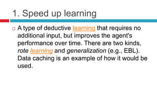
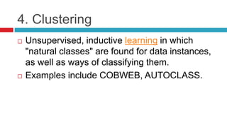
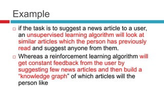
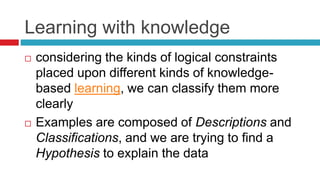
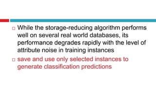
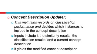
![2. Learning by taking advice
Deductive learning in which the system can
reason about new information added to its
knowledge base.
McCarthy proposed the "advice taker" which
was such a system, and TEIRESIAS [Davis,
1976] was the first such system.](https://image.slidesharecdn.com/learninginaislideshare-170919135830/85/Learning-in-AI-7-320.jpg)
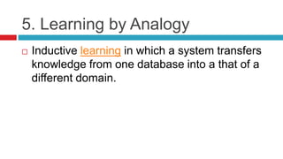
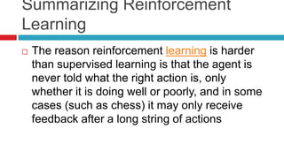
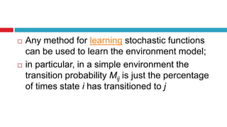
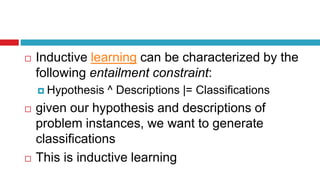
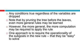
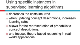
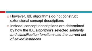
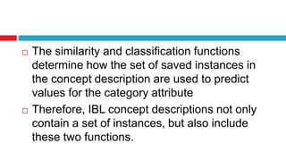
![To find HMAP, we apply Bayes' rule:
P(Hi | D) = [P(D | Hi) x P(Hi)] / P(D)
Since P(D) is fixed across the hypotheses, we
only need to maximize the numerator
The first term represents the probability that this
particular data set would be seen, given Hi as the
model of the world
The second is the prior probability assigned to the
model.](https://image.slidesharecdn.com/learninginaislideshare-170919135830/85/Learning-in-AI-15-320.jpg)
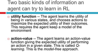
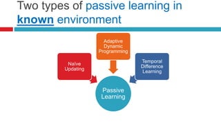
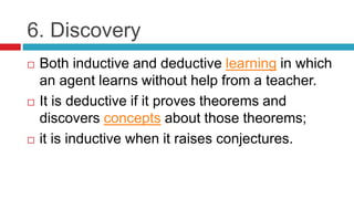
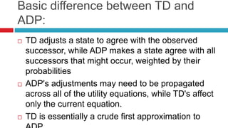
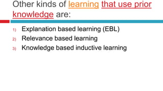
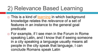
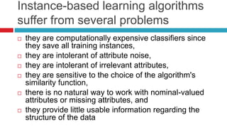
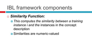
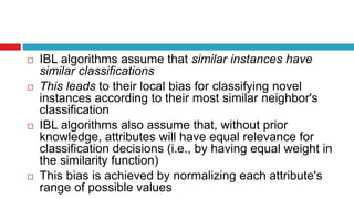
![1. Naive Updating
One simple updating method is the least mean
squares (LMS) approach [Widrow and Hoff,
1960].
It assumes that the observed reward-to-go of a
state in a sequence provides direct evidence
of the actual reward-to-go.
The approach is simply to keep the utility as a
running average of the rewards based upon
the number of times the state has been seen](https://image.slidesharecdn.com/learninginaislideshare-170919135830/85/Learning-in-AI-41-320.jpg)
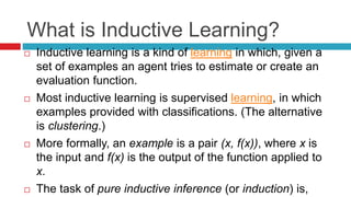
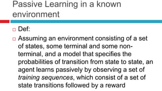
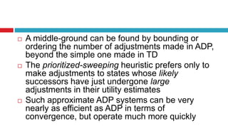
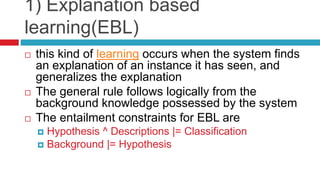
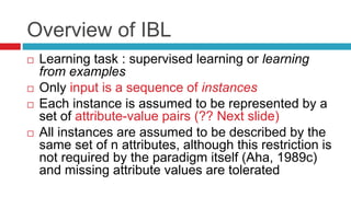
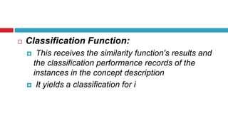
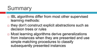
![ The idea generally is to define conditions that hold
over local transitions when the utility estimates are
correct, and then create update rules that nudge the
estimates toward this equation.
This approach will cause U(i) to converge to the
correct value if the learning rate parameter decreases
with the number of times a state has been visited
[Dayan, 1992].
In general, as the number of training sequences tends
to infinity, TD will converge on the same utilities as
ADP.](https://image.slidesharecdn.com/learninginaislideshare-170919135830/85/Learning-in-AI-47-320.jpg)
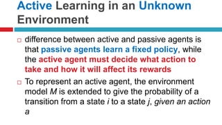
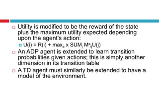
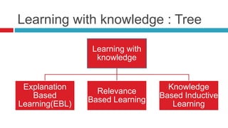


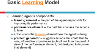
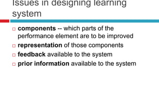
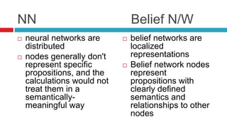
The document discusses various learning models in artificial intelligence, focusing on learning agents which consist of components like learning elements, performance elements, critics, and problem generators. It outlines different types of learning, including inductive learning, reinforcement learning, and the utilization of prior knowledge through methods like explanation-based learning and relevance-based learning. Additionally, it highlights the differences between neural networks and belief networks in terms of structure, representation, and learning processes.