The document provides guidance on statistics homework, specifically focusing on regression models and related calculations. It includes examples of linear regression for modeling the relationship between GPA and other factors, as well as residual analysis for assessing model fit. Additionally, it addresses fitting data from a proving ring experiment and comparing linear and quadratic models for better fit evaluation.

1.  For any help regarding Statistics Assignments
Visit: https://www.statisticshomeworkhelper.com
Email- info@statisticshomeworkhelper.com or call us at-+1 678 648 4277
Statistics Homework Helper

2. Problems from John A. Rice, Third Edition. [
C hapter.Secti on.Problem ]
1. 14.9.2. See Rscript/html Problem_l4_9_2.r 2. 14.9.4.
For modeling freshman GPA to depend linearly on high school GPA, a standard linear
regression model is:
Yi = /3o+ /31xi + ei, i = 1, 2, ... , n.
Suppose that different intercepts were to be allowed for femalses and males, and write the
model as
Yi= l p(i )/3F + IM(i)/3M + /31xi + e,;, i = 1, 2, ... , n.
where Jp(i) and JM(i) are indicator variables takingon values of Oand
1 according to whether the generder of the ith person is female or
male.
The design matrix for such a model will be
I Jp(l)
I
IM(l) X1
Jp(2) JM(2) x2
X=
lp(n) IM(n) Xn
LFemale -l
Xi
n
M
'L
"
,"
"
M ale i X
i
L M ale ,; Xi
'L
",
"n"l X
•
7
where np and nM are the number of femals and males, respectively. The regression model is
setup as
Note that xr X =
0
Statistics Homework Helper

3. 3. 14.9.6. The 4 weighings correspond to 4 outcomes of the dependent variable y
For the regression parameter vector
/3= [ W1 ]
W2
the design matrix is
-
1
X= [ 1 i
1 1
The regression model is
Y = X /3+ e
(b). The least squares estimates of w1 and w2 are given by
= [ 1
]
= (X Tx )- l x T y
W2
Note that
(XT X) = [ ] so
and
9
(XT Y ) = [ 11
] ,
SO = [ 1 3 1 3 ] X [ 1
1 ] =
9
[ l
l
f
3 ]
(c). The estimate of a 2 is given by the sum of squared residuals divided by n - 2, where 2 is the number of columns of
X which equals the number of regression parameters estimated.
The vector of least squares residuals is:
3
= [ = [
3
e
= [ =
: !
:
l t J
:
l tJ
y4 - f;4 7 - 20/3 1/ 3
From this we can compute
Statistics Homework Helper

4. Statistics Homework Helper

5. Problem_14_9_2.r
Peter
Thu Apr 30 21:21:38 2015
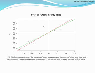
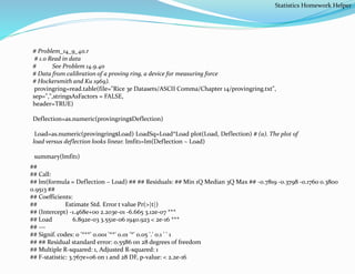
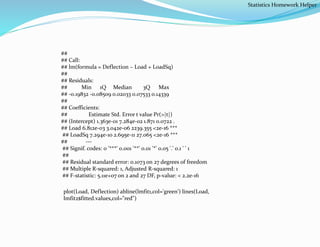
#Problem_14_9_2.r x=c(.34,1.38,-.64,.68,1.40,-.88,-.30, -1.18, .50, -1.75) y=c(.27,1.34,-.53,.35,1.28,-.98,0.72,-.81,.64,-1.59) # (a) Fit line y=a + bx
using lm() in r plot(x,y) lmfit1<-lm(y~x) summary(lmfit1)
## ## Call: ## lm(formula = y ~ x) ## ## Residuals: ## Min 1Q Median 3Q
Max ## -0.34954 -0.16556 -0.06363 0.08067 0.87278 ## ## Coefficients: ##
Estimate Std. Error t value Pr(>|t|) ## (Intercept) 0.1081 0.1156 0.935 0.377
## x 0.8697 0.1133 7.677 5.87e-05 *** ## --- ## Signif. codes: 0 '***' 0.001 '**'
0.01 '*' 0.05 '.' 0.1 ' ' 1 ## ## Residual standard error: 0.3654 on 8 degrees of
freedom ## Multiple R-squared: 0.8805, Adjusted R-squared: 0.8655 ## F-
statistic: 58.94 on 1 and 8 DF, p-value: 5.867e-05
abline(lmfit1,col='green') lmfit1$coefficients
## (Intercept) x ## 0.1081372 0.8697151
# (b) Fit line x=c+dy using lm() in r lmfit2<-lm(x~y) summary(lmfit2)
## ## Call: ## lm(formula = x ~ y) ## ## Residuals: ## Min 1Q Median 3Q Max ## -0.91406 -0.03117 0.07484 0.20963
0.44052 ## ## Coefficients: ## Estimate Std. Error t value Pr(>|t|) ## (Intercept) -0.1149 0.1250 -0.919 0.385 ## y 1.0124
0.1319 7.677 5.87e-05 *** ## --- ## Signif. codes: 0 '***' 0.001 '**' 0.01 '*' 0.05 '.' 0.1 ' ' 1 ## ## Residual standard error:
0.3942 on 8 degrees of freedom ## Multiple R-squared: 0.8805, Adjusted R-squared: 0.8655 ## F-statistic: 58.94 on 1 and
8 DF, p-value: 5.867e-05
lmfit2$coefficients
## (Intercept) y ## -0.1148545 1.0123846
# For x = b1 + b2y # we get the y vs x line as # y=-(b1/b2) + (1/b2)x abline(a=-
lmfit2$coefficients[1]/lmfit2$coefficients[2], b=(1/lmfit2$coefficients[2]), col="red") title(main="Y=a + bx
(Green) X=c+dy (Red)") abline(h=mean(y)); abline(v=mean(x)) abline(h=mean(y));abline(v=mean(x)) # Plot
horizontal/vertical lines at y/x means
Statistics Homework Helper

6. # (c). THe lines are not the same. The regression of y on x regresses toward the mean # of y (less steep slope) and
the regression of x on y regresses toward the mean of # x (which is less steep for x vs y, but more steep for y vs x)
Statistics Homework Helper

7. # Problem_14_9_40.r
# 1.0 Read in data
# See Problem 14.9.40
# Data from calibration of a proving ring, a device for measuring force
# Hockersmith and Ku 1969).
provingring=read.table(file="Rice 3e Datasets/ASCII Comma/Chapter 14/provingring.txt",
sep=",",stringsAsFactors = FALSE,
header=TRUE)
Deflection=as.numeric(provingring$Deflection)
Load=as.numeric(provingring$Load) LoadSq=Load*Load plot(Load, Deflection) # (a). The plot of
load versus deflection looks linear. lmfit1=lm(Deflection ~ Load)
summary(lmfit1)
##
## Call:
## lm(formula = Deflection ~ Load) ## ## Residuals: ## Min 1Q Median 3Q Max ## -0.7819 -0.3798 -0.1760 0.3800
0.9513 ##
## Coefficients:
## Estimate Std. Error t value Pr(>|t|)
## (Intercept) -1.468e+00 2.203e-01 -6.665 3.12e-07 ***
## Load 6.892e-03 3.551e-06 1940.923 < 2e-16 ***
## ---
## Signif. codes: 0 '***' 0.001 '**' 0.01 '*' 0.05 '.' 0.1 ' ' 1
## ## Residual standard error: 0.5586 on 28 degrees of freedom
## Multiple R-squared: 1, Adjusted R-squared: 1
## F-statistic: 3.767e+06 on 1 and 28 DF, p-value: < 2.2e-16
Statistics Homework Helper

8. plot(Load, Deflection) abline(lmfit1,col='green')
plot(lmfit1$residuals)
Statistics Homework Helper

9. plot(Load, lmfit1$residuals)
Statistics Homework Helper

10. # (b). The residuals from the linear fit show lack of fit
# The residuals are positive at the edges and negative in the middle of the Load values
# (c). Fit deflection as a quadratic function of load.
lmfit2=lm(Deflection ~ Load + LoadSq)
summary(lmfit2)
Statistics Homework Helper

11. ##
## Call:
## lm(formula = Deflection ~ Load + LoadSq)
##
## Residuals:
## Min 1Q Median 3Q Max
## -0.19832 -0.08509 0.02033 0.07533 0.14339
##
## Coefficients:
## Estimate Std. Error t value Pr(>|t|)
## (Intercept) 1.363e-01 7.284e-02 1.871 0.0722 .
## Load 6.812e-03 3.042e-06 2239.355 <2e-16 ***
## LoadSq 7.294e-10 2.695e-11 27.065 <2e-16 ***
## ---
## Signif. codes: 0 '***' 0.001 '**' 0.01 '*' 0.05 '.' 0.1 ' ' 1
##
## Residual standard error: 0.1073 on 27 degrees of freedom
## Multiple R-squared: 1, Adjusted R-squared: 1
## F-statistic: 5.11e+07 on 2 and 27 DF, p-value: < 2.2e-16
plot(Load, Deflection) abline(lmfit1,col='green') lines(Load,
lmfit2$fitted.values,col="red")
Statistics Homework Helper

12. plot(lmfit2$residuals)
Statistics Homework Helper

13. plot(Load, lmfit2$residuals) abline(h=0,col='gray')
Statistics Homework Helper

14. # The fit looks better. It is apparent that the variability across runs within a # given case of Load
is much lower than the variability across Loads # The errors in the measurements apparently
have two sources of variability.
Statistics Homework Helper