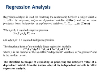
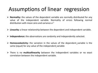
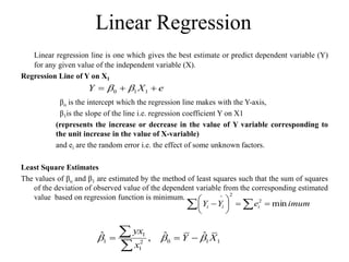
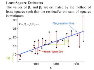
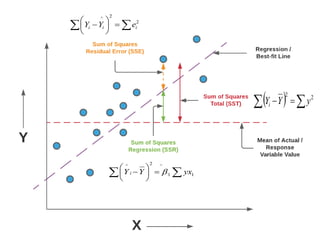
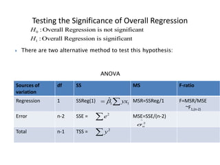
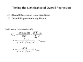
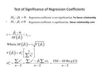
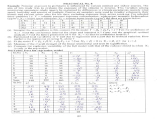
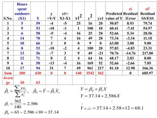
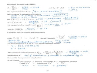
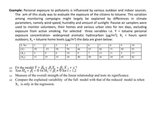
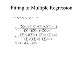
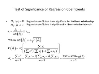
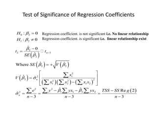
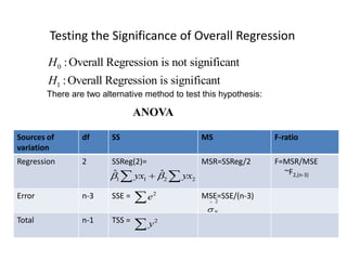
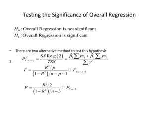
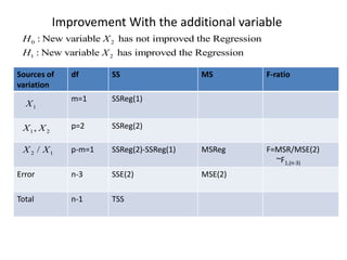
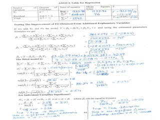
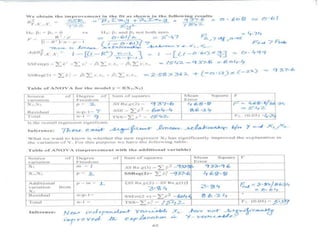
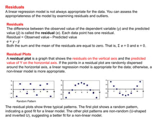
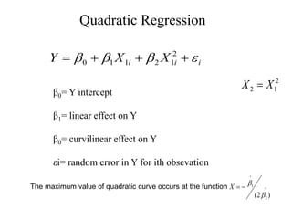
SlideShare a Scribd company logo
Dr. Pritpal Singh
Sr. Statistician
Department of Plant Breeding and Genetics
Regression Analysis
Regression analysis is used for modeling the relationship between a single variable
Y, called the response, output or dependent variable, (Effect) and one or more
predictor, input, independent or explanatory variables, X1, X2,…., Xp. (Cause)
When p=1, it is called simple regression
Y = β 0 + β1 X 1 + e
and when p> 1 it is called multiple regression.
The functional form of the multiple linear regression model is
Y = β 0 + β1 X 1 + β 2 X 2 +.. + β p X p + e
where p is the number of the so-called "independent" variables, or "regressors“ and
is the random error.
The statistical technique of estimating or predicting the unknown value of a
dependent variable from the known value of the independent variable is called
regression analysis.
Regression Analysis
Assumptions of linear regression
 Normality: the values of the dependent variable are normally distributed for any
value of the independent variable. Normality of errors following normal
distribution with mean zero and variance σ 2
 Linearity: a linear relationship between the dependent and independent variable.
 Independence: the observations are randomly and independently selected.
 Homoscedasticity: the variation in the values of the dependent variable is the
same (equal) for any value of the independent variable
 There is no multicollinearity between the independent variables or no exact
correlation between the independent variable.
Linear Regression
Linear regression line is one which gives the best estimate or predict dependent variable (Y)
for any given value of the independent variable (X).
Regression Line of Y on X1
βo is the intercept which the regression line makes with the Y-axis,
β1is the slope of the line i.e. regression coefficient Y on X1
(represents the increase or decrease in the value of Y variable corresponding to
the unit increase in the value of X-variable)
and ei are the random error i.e. the effect of some unknown factors.
Least Square Estimates
The values of βo and β1 are estimated by the method of least squares such that the sum of squares
of the deviation of observed value of the dependent variable from the corresponding estimated
value based on regression function is minimum.
1
1 0 1 1
2
1
ˆ ˆ ˆ
,
yx
Y X
x
  
  


0 1 1
Y X e
 
  
imum
e
Y
Y i
i
i min
2
2
^








 

Least Square Estimates
The values of βo and β1 are estimated by the method of
least squares such that the residual/errors sum of squares
is minimum
0 1 1
Y X e
 
  
 







 1
1
^
2
^
yx
Y
Y i 

 






 2
2
^
i
i
i e
Y
Y
  
 
 2
2
y
Y
Yi
Testing the Significance of Overall Regression
Sources of
variation
df SS MS F-ratio
Regression 1 SSReg(1) MSR=SSReg/1 F=MSR/MSE
~F1,(n-2)
Error n-2 SSE = MSE=SSE/(n-2)
Total n-1 TSS =
1 1
ˆ yx

 
2
y

2
e

 There are two alternative method to test this hypothesis:
ANOVA
0
1
: Overall Regression is not significant
: Overall Regression is significant
H
H
^
2
u

Testing the Significance of Overall Regression
Coefficient of Determination (R2)
 
1
1 1
2
. 2
ˆ
Re 1
Y X
yx
SS g
R
TSS y

 


0
1
: Overall Regression is not significant
: Overall Regression is significant
H
H
 
2
, 1
2
1 1
p n p
R p
F F
R n p
 

  
 
2
1, 2
2
1
1 2
n
R
F F
R n


 
Test of Significance of Regression Coefficients
.
 
   
 
 
1
2
1
1 1
2
1 2
1
2 2
1 1
2
ˆ 0
ˆ
ˆ ˆ
Where
1
ˆ ˆ
ˆ Re 1
ˆ
2 2 2
n
u
u
t t
SE
SE V
V
x
e y yx TSS SS g
n n n


 
 





 
 
  
 
 
 
  
  

  
0
:
0
:
1
1
1
0




H
H Regression coefficient. is not significant i.e. No linear relationship
Regression coefficient. is significant i.e. linear relationship exist
S.No.
Hours
spent
outdoors
(X1) Y
y
=Y-Y
x1=
X1-X1 x12 y
2 yx1
Predicted
value of Y
ei
Residual
/Error
ei2
Residual
SS/ESS
1 5 59 -4 -5 25 16 20 50.07 8.93 79.74
2 9 53 -10 -1 1 100 10 60.41 -7.41 54.97
3 6 58 -5 -4 16 25 20 52.66 5.34 28.56
4 14 70 7 4 16 49 28 73.34 -3.34 11.18
5 10 66 3 0 0 9 0 63.00 3.00 9.00
6 8 53 -10 -2 4 100 20 57.83 -4.83 23.31
7 13 56 -7 3 9 49 -21 70.76 -14.76 217.80
8 12 71 8 2 4 64 16 68.17 2.83 8.00
9 6 50 -13 -4 16 169 52 52.66 -2.66 7.05
10 17 94 31 7 49 961 217 81.10 12.90 166.36
Sum 100 630 0 0 140 1542 362 0 605.97
Avera
ge 10 63
1
1 0 1 1
2
1
ˆ ˆ ˆ
,
yx
Y X
x
  
  


14
.
37
10
586
.
2
63
586
.
2
140
362
0
1








^
12
^
1
0
1
.
68
12
58
.
2
14
.
37
586
.
2
14
.
37









X
Y
X
Y
X
Y 

Example: Personal exposure to pollutants is influenced by various outdoor and indoor sources.
The aim of this study was to evaluate the exposure of the citizens to toluene. This variation
among monitoring campaigns might largely be explained by differences in climate
parameters, namely wind speed, humidity and amount of sunlight. Passive air samplers were
used to monitor volunteers, their homes and various urban sites for ten days, excluding
exposure from active smoking. For selected three variables i.e. Y = toluene personal
exposure concentration- widespread aromatic hydrocarbon (µg/m3); X1 = hours spent
outdoors; X2 = toluene home levels (µg/m3) the data are given below:
(a) Fit the model Y  0  1X1  2 X 2  e ?
(b) Test H0  i  0 vs H1  i  0 for i  1,2
(c) Measure of the overall strength of the linear relationship and tests its significance.
(d) Compare the explained variability of the full model with that of the reduced model ie.when
X1 is only in the regression.
S. No 1 2 3 4 5 6 7 8 9 10
(Y) 59 53 58 70 66 53 56 71 50 91
(X1) 5 9 6 14 9 7 13 11 5 17
(X2) 31 35 35 34 40 50 36 34 45 42
Fitting of Multiple Regression
.
     
    
     
    
2
1 2 2 1 2
1 2
2 2
1 2 1 2
2
2 1 1 1 2
2 2
2 2
1 2 1 2
0 1 1 2 2
ˆ ,
ˆ
ˆ ˆ ˆ
yx x yx x x
x x x x
yx x yx x x
x x x x
Y X X


  






  
   
  
   
  
0 1 1 2 2
Y X X e
  
   
Test of Significance of Regression Coefficients
. 0 1
1 1
: 0
: 0
H
H




 
   
 
    
 
1
1 3
1
1 1
2
2
2
1 2
2 2
1 2 1 2
2 2
1 1 2 2
2
ˆ 0
ˆ
ˆ ˆ
Where
ˆ ˆ
ˆ ˆ Re 2
ˆ
3 3 3
n
u
u
t t
SE
SE V
x
V
x x x x
e y yx yx TSS SS g
n n n


 
 
 




 
 
 

 

 
  
  
  

  
   
Regression coefficient. is not significant i.e. No linear relationship
Regression coefficient. is significant i.e. linear relationship exist
Test of Significance of Regression Coefficients
0 2
1 2
: 0
: 0
H
H




 
   
 
    
 
2
2 3
2
2 2
2
1
2
2 2
2 2
1 2 1 2
2 2
1 1 2 2
2
ˆ 0
ˆ
ˆ ˆ
Where
ˆ ˆ
ˆ ˆ Re 2
ˆ
3 3 3
n
u
u
t t
SE
SE V
x
V
x x x x
e y yx yx TSS SS g
n n n


 
 
 




 
 
 

 

 
  
  
  

  
   
Regression coefficient. is significant i.e. linear relationship exist
Regression coefficient. is not significant i.e. No linear relationship
Sources of
variation
df SS MS F-ratio
Regression 2 SSReg(2)= MSR=SSReg/2 F=MSR/MSE
~F2,(n-3)
Error n-3 SSE = MSE=SSE/(n-3)
Total n-1 TSS =
1 1 2 2
ˆ ˆ
yx yx
 

 
2
y

2
e

0
1
:Overall Regression is not significant
:Overall Regression is significant
H
H
Testing the Significance of Overall Regression
There are two alternative method to test this hypothesis:
ANOVA
2
^
u

Testing the Significance of Overall Regression
• There are two alternative method to test this hypothesis:
2.
 
1 2
1 1 2 2
2
. 2
ˆ ˆ
Re 2
Y X X
yx yx
SS g
R
TSS y
 

 
 

0
1
: Overall Regression is not significant
: Overall Regression is significant
H
H
 
2
, 1
2
1 1
p n p
R p
F F
R n p
 

  
 
2
2, 3
2
2
1 3
n
R
F F
R n


 
Improvement With the additional variable
0 2
1 2
: New variable has not improved the Regression
: New variable has improved the Regression
H X
H X
Sources of
variation
df SS MS F-ratio
m=1 SSReg(1)
p=2 SSReg(2)
p-m=1 SSReg(2)-SSReg(1) MSReg F=MSR/MSE(2)
~F1,(n-3)
Error n-3 SSE(2) MSE(2)
Total n-1 TSS
1
X
1 2
,
X X
2 1
/
X X
Residuals
A linear regression model is not always appropriate for the data. You can assess the
appropriateness of the model by examining residuals and outliers.
Residuals
The difference between the observed value of the dependent variable (y) and the predicted
value (ŷ) is called the residual (e). Each data point has one residual.
Residual = Observed value - Predicted value
e = y - ŷ
Both the sum and the mean of the residuals are equal to zero. That is, Σ e = 0 and e = 0.
Residual Plots
A residual plot is a graph that shows the residuals on the vertical axis and the predicted
value of Y on the horizontal axis. If the points in a residual plot are randomly dispersed
around the horizontal axis, a linear regression model is appropriate for the data; otherwise, a
non-linear model is more appropriate.
The residual plots show three typical patterns. The first plot shows a random pattern,
indicating a good fit for a linear model. The other plot patterns are non-random (U-shaped
and inverted U), suggesting a better fit for a non-linear model.
Random Pattern
Quadratic Regression
i
i
i X
X
Y e


 


 2
1
2
1
1
0
β0= Y intercept
β1= linear effect on Y
β0= curvilinear effect on Y
εi= random error in Y for ith obsevation
The maximum value of quadratic curve occurs at the function ^
2
^
1
)
2
( 



X
2
1
2 X
X 
Quadratic Regression
^
2
^
1
)
2
( 



X
Fertilizer
(X) Yield (Y)
20 60
25 100
30 128
35 145
45 160
55 170
60 160
65 140
70 150
y = 1.4x + 71.77
R² = 0.544
0
20
40
60
80
100
120
140
160
180
0 20 40 60 80
Yield (Y)
Yield (Y)
Linear (Yield (Y))
y = -0.097x2 + 10.20x - 96.95
R² = 0.950
0
20
40
60
80
100
120
140
160
180
0 20 40 60 80
Yield (Y)
Yield (Y)
Poly. (Yield (Y))
Practical 9(a)
58
.
52
)
097
.
0
2
(
20
.
10
)
2
(
^
2
^
1 








X

More Related Content

Similar to regression analysis .ppt

Slideset Simple Linear Regression models.ppt
Slideset Simple Linear Regression models.pptSlideset Simple Linear Regression models.ppt
Slideset Simple Linear Regression models.ppt
rahulrkmgb09
 
lecture13.ppt
lecture13.pptlecture13.ppt
lecture13.ppt
WaqarTariq18
 
Regression.ppt basic introduction of regression with example
Regression.ppt basic introduction of regression with exampleRegression.ppt basic introduction of regression with example
Regression.ppt basic introduction of regression with example
shivshankarshiva98
 
Statistics
Statistics Statistics
Statistics
KafiPati
 
Regression
RegressionRegression
Regression
Sauravurp
 
Correlation by Neeraj Bhandari ( Surkhet.Nepal )
Correlation by Neeraj Bhandari ( Surkhet.Nepal )Correlation by Neeraj Bhandari ( Surkhet.Nepal )
Correlation by Neeraj Bhandari ( Surkhet.Nepal )Neeraj Bhandari
 
Regression
RegressionRegression
Regression
LavanyaK75
 
Regression
RegressionRegression
Linear regression.ppt
Linear regression.pptLinear regression.ppt
Linear regression.ppt
habtamu biazin
 
Simple Linear Regression
Simple Linear RegressionSimple Linear Regression
Simple Linear Regression
Sindhu Rumesh Kumar
 
linear Regression, multiple Regression and Annova
linear Regression, multiple Regression and Annovalinear Regression, multiple Regression and Annova
linear Regression, multiple Regression and Annova
Mansi Rastogi
 
Linear Regression
Linear RegressionLinear Regression
Linear Regression
Michael770443
 
REGRESSION ANALYSIS THEORY EXPLAINED HERE
REGRESSION ANALYSIS THEORY EXPLAINED HEREREGRESSION ANALYSIS THEORY EXPLAINED HERE
REGRESSION ANALYSIS THEORY EXPLAINED HERE
ShriramKargaonkar
 
Corr-and-Regress (1).ppt
Corr-and-Regress (1).pptCorr-and-Regress (1).ppt
Corr-and-Regress (1).ppt
MuhammadAftab89
 
Corr-and-Regress.ppt
Corr-and-Regress.pptCorr-and-Regress.ppt
Corr-and-Regress.ppt
BAGARAGAZAROMUALD2
 
Cr-and-Regress.ppt
Cr-and-Regress.pptCr-and-Regress.ppt
Cr-and-Regress.ppt
RidaIrfan10
 
Correlation & Regression for Statistics Social Science
Correlation & Regression for Statistics Social ScienceCorrelation & Regression for Statistics Social Science
Correlation & Regression for Statistics Social Science
ssuser71ac73
 
Corr-and-Regress.ppt
Corr-and-Regress.pptCorr-and-Regress.ppt
Corr-and-Regress.ppt
HarunorRashid74
 
Corr-and-Regress.ppt
Corr-and-Regress.pptCorr-and-Regress.ppt
Corr-and-Regress.ppt
krunal soni
 

Similar to regression analysis .ppt (20)

Slideset Simple Linear Regression models.ppt
Slideset Simple Linear Regression models.pptSlideset Simple Linear Regression models.ppt
Slideset Simple Linear Regression models.ppt
 
lecture13.ppt
lecture13.pptlecture13.ppt
lecture13.ppt
 
Regression.ppt basic introduction of regression with example
Regression.ppt basic introduction of regression with exampleRegression.ppt basic introduction of regression with example
Regression.ppt basic introduction of regression with example
 
Statistics
Statistics Statistics
Statistics
 
Regression
RegressionRegression
Regression
 
Correlation by Neeraj Bhandari ( Surkhet.Nepal )
Correlation by Neeraj Bhandari ( Surkhet.Nepal )Correlation by Neeraj Bhandari ( Surkhet.Nepal )
Correlation by Neeraj Bhandari ( Surkhet.Nepal )
 
Regression
RegressionRegression
Regression
 
Regression
RegressionRegression
Regression
 
Linear regression.ppt
Linear regression.pptLinear regression.ppt
Linear regression.ppt
 
Simple Linear Regression
Simple Linear RegressionSimple Linear Regression
Simple Linear Regression
 
linear Regression, multiple Regression and Annova
linear Regression, multiple Regression and Annovalinear Regression, multiple Regression and Annova
linear Regression, multiple Regression and Annova
 
Linear Regression
Linear RegressionLinear Regression
Linear Regression
 
REGRESSION ANALYSIS THEORY EXPLAINED HERE
REGRESSION ANALYSIS THEORY EXPLAINED HEREREGRESSION ANALYSIS THEORY EXPLAINED HERE
REGRESSION ANALYSIS THEORY EXPLAINED HERE
 
Regression analysis
Regression analysisRegression analysis
Regression analysis
 
Corr-and-Regress (1).ppt
Corr-and-Regress (1).pptCorr-and-Regress (1).ppt
Corr-and-Regress (1).ppt
 
Corr-and-Regress.ppt
Corr-and-Regress.pptCorr-and-Regress.ppt
Corr-and-Regress.ppt
 
Cr-and-Regress.ppt
Cr-and-Regress.pptCr-and-Regress.ppt
Cr-and-Regress.ppt
 
Correlation & Regression for Statistics Social Science
Correlation & Regression for Statistics Social ScienceCorrelation & Regression for Statistics Social Science
Correlation & Regression for Statistics Social Science
 
Corr-and-Regress.ppt
Corr-and-Regress.pptCorr-and-Regress.ppt
Corr-and-Regress.ppt
 
Corr-and-Regress.ppt
Corr-and-Regress.pptCorr-and-Regress.ppt
Corr-and-Regress.ppt
 

Recently uploaded

Lapbook sobre os Regimes Totalitários.pdf
Lapbook sobre os Regimes Totalitários.pdfLapbook sobre os Regimes Totalitários.pdf
Lapbook sobre os Regimes Totalitários.pdf
Jean Carlos Nunes Paixão
 
Honest Reviews of Tim Han LMA Course Program.pptx
Honest Reviews of Tim Han LMA Course Program.pptxHonest Reviews of Tim Han LMA Course Program.pptx
Honest Reviews of Tim Han LMA Course Program.pptx
timhan337
 
Digital Tools and AI for Teaching Learning and Research
Digital Tools and AI for Teaching Learning and ResearchDigital Tools and AI for Teaching Learning and Research
Digital Tools and AI for Teaching Learning and Research
Vikramjit Singh
 
Guidance_and_Counselling.pdf B.Ed. 4th Semester
Guidance_and_Counselling.pdf B.Ed. 4th SemesterGuidance_and_Counselling.pdf B.Ed. 4th Semester
Guidance_and_Counselling.pdf B.Ed. 4th Semester
Atul Kumar Singh
 
Welcome to TechSoup New Member Orientation and Q&A (May 2024).pdf
Welcome to TechSoup   New Member Orientation and Q&A (May 2024).pdfWelcome to TechSoup   New Member Orientation and Q&A (May 2024).pdf
Welcome to TechSoup New Member Orientation and Q&A (May 2024).pdf
TechSoup
 
The Accursed House by Émile Gaboriau.pptx
The Accursed House by Émile Gaboriau.pptxThe Accursed House by Émile Gaboriau.pptx
The Accursed House by Émile Gaboriau.pptx
DhatriParmar
 
Mule 4.6 & Java 17 Upgrade | MuleSoft Mysore Meetup #46
Mule 4.6 & Java 17 Upgrade | MuleSoft Mysore Meetup #46Mule 4.6 & Java 17 Upgrade | MuleSoft Mysore Meetup #46
Mule 4.6 & Java 17 Upgrade | MuleSoft Mysore Meetup #46
MysoreMuleSoftMeetup
 
Introduction to AI for Nonprofits with Tapp Network
Introduction to AI for Nonprofits with Tapp NetworkIntroduction to AI for Nonprofits with Tapp Network
Introduction to AI for Nonprofits with Tapp Network
TechSoup
 
Unit 2- Research Aptitude (UGC NET Paper I).pdf
Unit 2- Research Aptitude (UGC NET Paper I).pdfUnit 2- Research Aptitude (UGC NET Paper I).pdf
Unit 2- Research Aptitude (UGC NET Paper I).pdf
Thiyagu K
 
Biological Screening of Herbal Drugs in detailed.
Biological Screening of Herbal Drugs in detailed.Biological Screening of Herbal Drugs in detailed.
Biological Screening of Herbal Drugs in detailed.
Ashokrao Mane college of Pharmacy Peth-Vadgaon
 
Thesis Statement for students diagnonsed withADHD.ppt
Thesis Statement for students diagnonsed withADHD.pptThesis Statement for students diagnonsed withADHD.ppt
Thesis Statement for students diagnonsed withADHD.ppt
EverAndrsGuerraGuerr
 
CACJapan - GROUP Presentation 1- Wk 4.pdf
CACJapan - GROUP Presentation 1- Wk 4.pdfCACJapan - GROUP Presentation 1- Wk 4.pdf
CACJapan - GROUP Presentation 1- Wk 4.pdf
camakaiclarkmusic
 
Additional Benefits for Employee Website.pdf
Additional Benefits for Employee Website.pdfAdditional Benefits for Employee Website.pdf
Additional Benefits for Employee Website.pdf
joachimlavalley1
 
Synthetic Fiber Construction in lab .pptx
Synthetic Fiber Construction in lab .pptxSynthetic Fiber Construction in lab .pptx
Synthetic Fiber Construction in lab .pptx
Pavel ( NSTU)
 
Home assignment II on Spectroscopy 2024 Answers.pdf
Home assignment II on Spectroscopy 2024 Answers.pdfHome assignment II on Spectroscopy 2024 Answers.pdf
Home assignment II on Spectroscopy 2024 Answers.pdf
Tamralipta Mahavidyalaya
 
special B.ed 2nd year old paper_20240531.pdf
special B.ed 2nd year old paper_20240531.pdfspecial B.ed 2nd year old paper_20240531.pdf
special B.ed 2nd year old paper_20240531.pdf
Special education needs
 
TESDA TM1 REVIEWER FOR NATIONAL ASSESSMENT WRITTEN AND ORAL QUESTIONS WITH A...
TESDA TM1 REVIEWER  FOR NATIONAL ASSESSMENT WRITTEN AND ORAL QUESTIONS WITH A...TESDA TM1 REVIEWER  FOR NATIONAL ASSESSMENT WRITTEN AND ORAL QUESTIONS WITH A...
TESDA TM1 REVIEWER FOR NATIONAL ASSESSMENT WRITTEN AND ORAL QUESTIONS WITH A...
EugeneSaldivar
 
Language Across the Curriculm LAC B.Ed.
Language Across the  Curriculm LAC B.Ed.Language Across the  Curriculm LAC B.Ed.
Language Across the Curriculm LAC B.Ed.
Atul Kumar Singh
 
Polish students' mobility in the Czech Republic
Polish students' mobility in the Czech RepublicPolish students' mobility in the Czech Republic
Polish students' mobility in the Czech Republic
Anna Sz.
 
Sha'Carri Richardson Presentation 202345
Sha'Carri Richardson Presentation 202345Sha'Carri Richardson Presentation 202345
Sha'Carri Richardson Presentation 202345
beazzy04
 

Recently uploaded (20)

Lapbook sobre os Regimes Totalitários.pdf
Lapbook sobre os Regimes Totalitários.pdfLapbook sobre os Regimes Totalitários.pdf
Lapbook sobre os Regimes Totalitários.pdf
 
Honest Reviews of Tim Han LMA Course Program.pptx
Honest Reviews of Tim Han LMA Course Program.pptxHonest Reviews of Tim Han LMA Course Program.pptx
Honest Reviews of Tim Han LMA Course Program.pptx
 
Digital Tools and AI for Teaching Learning and Research
Digital Tools and AI for Teaching Learning and ResearchDigital Tools and AI for Teaching Learning and Research
Digital Tools and AI for Teaching Learning and Research
 
Guidance_and_Counselling.pdf B.Ed. 4th Semester
Guidance_and_Counselling.pdf B.Ed. 4th SemesterGuidance_and_Counselling.pdf B.Ed. 4th Semester
Guidance_and_Counselling.pdf B.Ed. 4th Semester
 
Welcome to TechSoup New Member Orientation and Q&A (May 2024).pdf
Welcome to TechSoup   New Member Orientation and Q&A (May 2024).pdfWelcome to TechSoup   New Member Orientation and Q&A (May 2024).pdf
Welcome to TechSoup New Member Orientation and Q&A (May 2024).pdf
 
The Accursed House by Émile Gaboriau.pptx
The Accursed House by Émile Gaboriau.pptxThe Accursed House by Émile Gaboriau.pptx
The Accursed House by Émile Gaboriau.pptx
 
Mule 4.6 & Java 17 Upgrade | MuleSoft Mysore Meetup #46
Mule 4.6 & Java 17 Upgrade | MuleSoft Mysore Meetup #46Mule 4.6 & Java 17 Upgrade | MuleSoft Mysore Meetup #46
Mule 4.6 & Java 17 Upgrade | MuleSoft Mysore Meetup #46
 
Introduction to AI for Nonprofits with Tapp Network
Introduction to AI for Nonprofits with Tapp NetworkIntroduction to AI for Nonprofits with Tapp Network
Introduction to AI for Nonprofits with Tapp Network
 
Unit 2- Research Aptitude (UGC NET Paper I).pdf
Unit 2- Research Aptitude (UGC NET Paper I).pdfUnit 2- Research Aptitude (UGC NET Paper I).pdf
Unit 2- Research Aptitude (UGC NET Paper I).pdf
 
Biological Screening of Herbal Drugs in detailed.
Biological Screening of Herbal Drugs in detailed.Biological Screening of Herbal Drugs in detailed.
Biological Screening of Herbal Drugs in detailed.
 
Thesis Statement for students diagnonsed withADHD.ppt
Thesis Statement for students diagnonsed withADHD.pptThesis Statement for students diagnonsed withADHD.ppt
Thesis Statement for students diagnonsed withADHD.ppt
 
CACJapan - GROUP Presentation 1- Wk 4.pdf
CACJapan - GROUP Presentation 1- Wk 4.pdfCACJapan - GROUP Presentation 1- Wk 4.pdf
CACJapan - GROUP Presentation 1- Wk 4.pdf
 
Additional Benefits for Employee Website.pdf
Additional Benefits for Employee Website.pdfAdditional Benefits for Employee Website.pdf
Additional Benefits for Employee Website.pdf
 
Synthetic Fiber Construction in lab .pptx
Synthetic Fiber Construction in lab .pptxSynthetic Fiber Construction in lab .pptx
Synthetic Fiber Construction in lab .pptx
 
Home assignment II on Spectroscopy 2024 Answers.pdf
Home assignment II on Spectroscopy 2024 Answers.pdfHome assignment II on Spectroscopy 2024 Answers.pdf
Home assignment II on Spectroscopy 2024 Answers.pdf
 
special B.ed 2nd year old paper_20240531.pdf
special B.ed 2nd year old paper_20240531.pdfspecial B.ed 2nd year old paper_20240531.pdf
special B.ed 2nd year old paper_20240531.pdf
 
TESDA TM1 REVIEWER FOR NATIONAL ASSESSMENT WRITTEN AND ORAL QUESTIONS WITH A...
TESDA TM1 REVIEWER  FOR NATIONAL ASSESSMENT WRITTEN AND ORAL QUESTIONS WITH A...TESDA TM1 REVIEWER  FOR NATIONAL ASSESSMENT WRITTEN AND ORAL QUESTIONS WITH A...
TESDA TM1 REVIEWER FOR NATIONAL ASSESSMENT WRITTEN AND ORAL QUESTIONS WITH A...
 
Language Across the Curriculm LAC B.Ed.
Language Across the  Curriculm LAC B.Ed.Language Across the  Curriculm LAC B.Ed.
Language Across the Curriculm LAC B.Ed.
 
Polish students' mobility in the Czech Republic
Polish students' mobility in the Czech RepublicPolish students' mobility in the Czech Republic
Polish students' mobility in the Czech Republic
 
Sha'Carri Richardson Presentation 202345
Sha'Carri Richardson Presentation 202345Sha'Carri Richardson Presentation 202345
Sha'Carri Richardson Presentation 202345
 

regression analysis .ppt

  • 1. Dr. Pritpal Singh Sr. Statistician Department of Plant Breeding and Genetics Regression Analysis
  • 2. Regression analysis is used for modeling the relationship between a single variable Y, called the response, output or dependent variable, (Effect) and one or more predictor, input, independent or explanatory variables, X1, X2,…., Xp. (Cause) When p=1, it is called simple regression Y = β 0 + β1 X 1 + e and when p> 1 it is called multiple regression. The functional form of the multiple linear regression model is Y = β 0 + β1 X 1 + β 2 X 2 +.. + β p X p + e where p is the number of the so-called "independent" variables, or "regressors“ and is the random error. The statistical technique of estimating or predicting the unknown value of a dependent variable from the known value of the independent variable is called regression analysis. Regression Analysis
  • 3. Assumptions of linear regression  Normality: the values of the dependent variable are normally distributed for any value of the independent variable. Normality of errors following normal distribution with mean zero and variance σ 2  Linearity: a linear relationship between the dependent and independent variable.  Independence: the observations are randomly and independently selected.  Homoscedasticity: the variation in the values of the dependent variable is the same (equal) for any value of the independent variable  There is no multicollinearity between the independent variables or no exact correlation between the independent variable.
  • 4. Linear Regression Linear regression line is one which gives the best estimate or predict dependent variable (Y) for any given value of the independent variable (X). Regression Line of Y on X1 βo is the intercept which the regression line makes with the Y-axis, β1is the slope of the line i.e. regression coefficient Y on X1 (represents the increase or decrease in the value of Y variable corresponding to the unit increase in the value of X-variable) and ei are the random error i.e. the effect of some unknown factors. Least Square Estimates The values of βo and β1 are estimated by the method of least squares such that the sum of squares of the deviation of observed value of the dependent variable from the corresponding estimated value based on regression function is minimum. 1 1 0 1 1 2 1 ˆ ˆ ˆ , yx Y X x         0 1 1 Y X e      imum e Y Y i i i min 2 2 ^           
  • 5. Least Square Estimates The values of βo and β1 are estimated by the method of least squares such that the residual/errors sum of squares is minimum 0 1 1 Y X e     
  • 6.           1 1 ^ 2 ^ yx Y Y i            2 2 ^ i i i e Y Y       2 2 y Y Yi
  • 7. Testing the Significance of Overall Regression Sources of variation df SS MS F-ratio Regression 1 SSReg(1) MSR=SSReg/1 F=MSR/MSE ~F1,(n-2) Error n-2 SSE = MSE=SSE/(n-2) Total n-1 TSS = 1 1 ˆ yx    2 y  2 e   There are two alternative method to test this hypothesis: ANOVA 0 1 : Overall Regression is not significant : Overall Regression is significant H H ^ 2 u 
  • 8. Testing the Significance of Overall Regression Coefficient of Determination (R2)   1 1 1 2 . 2 ˆ Re 1 Y X yx SS g R TSS y      0 1 : Overall Regression is not significant : Overall Regression is significant H H   2 , 1 2 1 1 p n p R p F F R n p         2 1, 2 2 1 1 2 n R F F R n    
  • 9. Test of Significance of Regression Coefficients .           1 2 1 1 1 2 1 2 1 2 2 1 1 2 ˆ 0 ˆ ˆ ˆ Where 1 ˆ ˆ ˆ Re 1 ˆ 2 2 2 n u u t t SE SE V V x e y yx TSS SS g n n n                                   0 : 0 : 1 1 1 0     H H Regression coefficient. is not significant i.e. No linear relationship Regression coefficient. is significant i.e. linear relationship exist
  • 10.
  • 11. S.No. Hours spent outdoors (X1) Y y =Y-Y x1= X1-X1 x12 y 2 yx1 Predicted value of Y ei Residual /Error ei2 Residual SS/ESS 1 5 59 -4 -5 25 16 20 50.07 8.93 79.74 2 9 53 -10 -1 1 100 10 60.41 -7.41 54.97 3 6 58 -5 -4 16 25 20 52.66 5.34 28.56 4 14 70 7 4 16 49 28 73.34 -3.34 11.18 5 10 66 3 0 0 9 0 63.00 3.00 9.00 6 8 53 -10 -2 4 100 20 57.83 -4.83 23.31 7 13 56 -7 3 9 49 -21 70.76 -14.76 217.80 8 12 71 8 2 4 64 16 68.17 2.83 8.00 9 6 50 -13 -4 16 169 52 52.66 -2.66 7.05 10 17 94 31 7 49 961 217 81.10 12.90 166.36 Sum 100 630 0 0 140 1542 362 0 605.97 Avera ge 10 63 1 1 0 1 1 2 1 ˆ ˆ ˆ , yx Y X x         14 . 37 10 586 . 2 63 586 . 2 140 362 0 1         ^ 12 ^ 1 0 1 . 68 12 58 . 2 14 . 37 586 . 2 14 . 37          X Y X Y X Y  
  • 12.
  • 13.
  • 14. Example: Personal exposure to pollutants is influenced by various outdoor and indoor sources. The aim of this study was to evaluate the exposure of the citizens to toluene. This variation among monitoring campaigns might largely be explained by differences in climate parameters, namely wind speed, humidity and amount of sunlight. Passive air samplers were used to monitor volunteers, their homes and various urban sites for ten days, excluding exposure from active smoking. For selected three variables i.e. Y = toluene personal exposure concentration- widespread aromatic hydrocarbon (µg/m3); X1 = hours spent outdoors; X2 = toluene home levels (µg/m3) the data are given below: (a) Fit the model Y  0  1X1  2 X 2  e ? (b) Test H0  i  0 vs H1  i  0 for i  1,2 (c) Measure of the overall strength of the linear relationship and tests its significance. (d) Compare the explained variability of the full model with that of the reduced model ie.when X1 is only in the regression. S. No 1 2 3 4 5 6 7 8 9 10 (Y) 59 53 58 70 66 53 56 71 50 91 (X1) 5 9 6 14 9 7 13 11 5 17 (X2) 31 35 35 34 40 50 36 34 45 42
  • 15. Fitting of Multiple Regression .                       2 1 2 2 1 2 1 2 2 2 1 2 1 2 2 2 1 1 1 2 2 2 2 2 1 2 1 2 0 1 1 2 2 ˆ , ˆ ˆ ˆ ˆ yx x yx x x x x x x yx x yx x x x x x x Y X X                             0 1 1 2 2 Y X X e       
  • 16. Test of Significance of Regression Coefficients . 0 1 1 1 : 0 : 0 H H                    1 1 3 1 1 1 2 2 2 1 2 2 2 1 2 1 2 2 2 1 1 2 2 2 ˆ 0 ˆ ˆ ˆ Where ˆ ˆ ˆ ˆ Re 2 ˆ 3 3 3 n u u t t SE SE V x V x x x x e y yx yx TSS SS g n n n                                          Regression coefficient. is not significant i.e. No linear relationship Regression coefficient. is significant i.e. linear relationship exist
  • 17. Test of Significance of Regression Coefficients 0 2 1 2 : 0 : 0 H H                    2 2 3 2 2 2 2 1 2 2 2 2 2 1 2 1 2 2 2 1 1 2 2 2 ˆ 0 ˆ ˆ ˆ Where ˆ ˆ ˆ ˆ Re 2 ˆ 3 3 3 n u u t t SE SE V x V x x x x e y yx yx TSS SS g n n n                                          Regression coefficient. is significant i.e. linear relationship exist Regression coefficient. is not significant i.e. No linear relationship
  • 18. Sources of variation df SS MS F-ratio Regression 2 SSReg(2)= MSR=SSReg/2 F=MSR/MSE ~F2,(n-3) Error n-3 SSE = MSE=SSE/(n-3) Total n-1 TSS = 1 1 2 2 ˆ ˆ yx yx      2 y  2 e  0 1 :Overall Regression is not significant :Overall Regression is significant H H Testing the Significance of Overall Regression There are two alternative method to test this hypothesis: ANOVA 2 ^ u 
  • 19. Testing the Significance of Overall Regression • There are two alternative method to test this hypothesis: 2.   1 2 1 1 2 2 2 . 2 ˆ ˆ Re 2 Y X X yx yx SS g R TSS y         0 1 : Overall Regression is not significant : Overall Regression is significant H H   2 , 1 2 1 1 p n p R p F F R n p         2 2, 3 2 2 1 3 n R F F R n    
  • 20. Improvement With the additional variable 0 2 1 2 : New variable has not improved the Regression : New variable has improved the Regression H X H X Sources of variation df SS MS F-ratio m=1 SSReg(1) p=2 SSReg(2) p-m=1 SSReg(2)-SSReg(1) MSReg F=MSR/MSE(2) ~F1,(n-3) Error n-3 SSE(2) MSE(2) Total n-1 TSS 1 X 1 2 , X X 2 1 / X X
  • 21.
  • 22.
  • 23. Residuals A linear regression model is not always appropriate for the data. You can assess the appropriateness of the model by examining residuals and outliers. Residuals The difference between the observed value of the dependent variable (y) and the predicted value (ŷ) is called the residual (e). Each data point has one residual. Residual = Observed value - Predicted value e = y - ŷ Both the sum and the mean of the residuals are equal to zero. That is, Σ e = 0 and e = 0. Residual Plots A residual plot is a graph that shows the residuals on the vertical axis and the predicted value of Y on the horizontal axis. If the points in a residual plot are randomly dispersed around the horizontal axis, a linear regression model is appropriate for the data; otherwise, a non-linear model is more appropriate. The residual plots show three typical patterns. The first plot shows a random pattern, indicating a good fit for a linear model. The other plot patterns are non-random (U-shaped and inverted U), suggesting a better fit for a non-linear model. Random Pattern
  • 24. Quadratic Regression i i i X X Y e        2 1 2 1 1 0 β0= Y intercept β1= linear effect on Y β0= curvilinear effect on Y εi= random error in Y for ith obsevation The maximum value of quadratic curve occurs at the function ^ 2 ^ 1 ) 2 (     X 2 1 2 X X 
  • 26. Fertilizer (X) Yield (Y) 20 60 25 100 30 128 35 145 45 160 55 170 60 160 65 140 70 150 y = 1.4x + 71.77 R² = 0.544 0 20 40 60 80 100 120 140 160 180 0 20 40 60 80 Yield (Y) Yield (Y) Linear (Yield (Y)) y = -0.097x2 + 10.20x - 96.95 R² = 0.950 0 20 40 60 80 100 120 140 160 180 0 20 40 60 80 Yield (Y) Yield (Y) Poly. (Yield (Y)) Practical 9(a) 58 . 52 ) 097 . 0 2 ( 20 . 10 ) 2 ( ^ 2 ^ 1          X