The document covers the fundamentals of linear regression and multiple linear regression, including definitions, methods to fit the regression line, and how to make predictions based on relationships between dependent and independent variables. It discusses real-world applications, examples of data analysis, and various components such as slope, intercept, and error measurement, emphasizing the importance of linearity in relationships. Additionally, it highlights the advantages and limitations of linear regression and provides insights into its practical usage in fields like real estate and medical research.

1. Linear Regression & Multiple
Linear Regression

2. STA6166-RegBasics 2
Lecture Outcomes
• What is Regression?
• Real World Examples
• The Line, the Slope and the Intercept
• How is a Simple Linear Regression Analysis done?
• Plotting
• Fitting the Line
• Finding the best Line

3. What is Linear Regression?
• Definition:
Linear regression is a statistical method used to model the
relationship between a dependent variable and one or more
independent variables.
• Regression is a statistical procedure that determines the equation for
the straight line that best fits a specific set of data.

5. Goal:
• We want to draw a straight line that best fits the data points, so we
can predict values for one variable based on the other(s).
• The goal of linear regression is to find the line that best fits the data
and can be used for prediction.

6. Real-World Example
• Scenario: Predicting house prices
• Independent Variable (X): Square footage of a house
• Dependent Variable (Y): Price of the house
• Question: How can we predict the price of a house based on its size?
Linear regression helps us understand this relationship.

7. Real-Life Example-II
• Scenario:
Imagine you want to predict a student's score on a test based on the
number of hours they studied.
• Independent variable (x): Number of hours studied
• Dependent variable (y): Test score
• The question:
Can we predict the test score by knowing the number of hours
studied?

8. Simple Linear Regression
• Equation for a Straight Line:
The equation for a straight line is:
y=β0+β1 x i.e y=mx+c
⋅
Where:
• y = predicted value (test score)
• x = independent variable (hours studied)
• β0​= intercept (the point where the line crosses the y-axis)
• β1​= slope (how much y changes for each change in x)

9. Understanding the Slope and Intercept
• Intercept (β0​
): This is the value of y when x=0. In our example, it's the
predicted score when no hours are studied. This is where the line
crosses the Y-axis
• Slope (β1​
):
This shows how much the dependent variable (y) changes for each
unit change in the independent variable (x).
•
In our example, it tells us how much the test score increases for each
additional hour of study.
The ‘c’
The ‘m’

11. The Straight Line
11
• Any straight line can be represented by an equation of the form Y = bX
+ a, where b and a are constants.
• The value of b is called the slope constant and determines the
direction and degree to which the line is tilted.
• The value of a is called the Y-intercept and determines the point
where the line crosses the Y-axis.

12. Visualizing Linear Regression
• Graph Example:
• X-axis: Hours studied (independent variable)
• Y-axis: Test score (dependent variable)
• Scatter Plot:
Plot data points showing hours studied versus test scores.
• Regression Line:
The straight line drawn through the points that best represents the
relationship between hours studied and test score.

13. How Does Linear Regression Work?
• Objective:
Find the line that best fits the data by minimizing the difference
between actual values and predicted values.
• How do we fit the line?
• We use a method called Least Squares to minimize the error (the difference
between actual and predicted points).
• Error (Residual):
The difference between the observed value (real test score) and the
predicted value (value on the line).

14. How Do We Find the Best-Fitting Line?
• Method: Least Squares Method
• This method minimizes the sum of the squared differences between the
observed (actual) values and the predicted values.
• Formula for minimizing:
• where Yi are the actual values and are the predicted values.

15. Evaluating the Model
•Mean Squared Error (MSE):
•This measures the average of the squared differences between actual and predicted
values.
•The lower the MSE, the better the model.

16. Steps in Linear Regression
1.Collect data:
Gather data for the dependent and independent variables (e.g., hours
studied and test scores).
2.Plot the data:
Create a scatter plot to visualize the relationship between variables.
3.Fit the line:
Use linear regression to find the line that best fits the data.
4.Make predictions:
Once the line is fitted, use it to make predictions about new data (e.g.,
predict test scores based on hours studied).

17. Linear Regression (cont.)
17
• How well a set of data points fits a straight line can be measured by
calculating the distance between the data points and the line.
• The total error between the data points and the line is obtained by
squaring each distance and then summing the squared values.
• The regression equation is designed to produce the minimum sum of
squared errors.

18. STA6166-RegBasics 18
An operations supervisor measured how long it takes one of her drivers to put 1, 2, 3 and 4
cases of soft drink into a soft drink machine. In this case the levels of the explanatory variable,
X are {1,2,3,4}, and she controls them. She might repeat the measurement a couple of times at
each level of X. A scatter plot of the resulting data might look like:

19. STA6166-RegBasics 19
A forestry graduate student makes wrapping paper out of different percentages
of hardwood then measure its tensile strength. He has the freedom to choose at
the beginning of the study to have only five percentages to work with, say {5%,
10%, 15%, 20%, and 25%}. A scatter plot of the resulting data might look like:

20. STA6166-RegBasics 20
A farm manager is interested in the relationship between litter size and average
litter weight (average newborn piglet weight). She examines the farm records
over the last couple of years and records the litter size and average weight for all
births. A plot of the data pairs looks like the following:

21. STA6166-RegBasics 21
A farm operations student is interested in the relationship between maintenance
cost and age of farm tractors. He performs a telephone interview survey of the 52
commercial potato growers in Putnam County, FL. One part of the questionnaire
provides information on tractor age and 1995 maintenance cost (fuel, lubricants,
repairs, etc). A plot of these data might look like:

22. STA6166-RegBasics 22
• What is the association between Y and X?
• How can changes in Y be explained by changes in X?
• What are the functional relationships between Y and X?
A functional relationship is symbolically written as:
)
(X
f
Y 
Eq: 1
Example: A proportional
relationship (e.g. fish weight to
length).
X
b
Y 1

b1 is the slope of the line.
Questions needing answers.

23. STA6166-RegBasics 23
b0 is the intercept,
b1 is the slope.
X
b
b
Y 1
0 

Example: Linear relationship (e.g. Y=cholesterol
versus X=age)

24. Problem Statement
•

25. Linear Regression: Fitting a Line
𝒚 =(𝒎𝒙 + 𝒃)

26. Which Line Best Fits the data points (This One)

27. Which Line Best Fits the data points (Or This One)

28. Which Line Best Fits the data points (Or This One)

29. Finding out the best line
The line which minimizes the sum of square errors

30. Linear Regression (Example)
• Find the best line that fits the following data points:
X 1 2 3 4 5 6 7
Y 1.5 3.8 6.7 9.0 11.2 13.6 16

31. Linear Regression (Example): Plot

32. Linear Regression (Example)
X Y XY X2
1 1.5 1.5 1
2 3.8 7.6 4
3 6.7 20.1 9
4 9.0 36 16
5 11.2 56 25
6 13.6 81.6 36
7 16 112 49
=28 61.8 314.8 =140

33. Linear Regression (Example)
•
• =-0.8285
• →

34. Linear Regression (Example)

35. Linear Regression (Example)
• → =3.99
• → =11.22
• → =16.04

36. Equations Governing Linear Regression

37. Finding out the best line
The line which minimizes the sum of square errors

38. Example (Home Work)
• The iodine value (x) is the amount of iodine necessary to saturate a
sample of 100 g of oil. Fit the simple linear regression model to this
data.

39. Multiple Linear Regression
• Boston Housing Data:

40. Multiple Linear Regression
• Titanic Data:

41. Multiple Linear Regression
• Iris Data:

42. Multiple Linear Regression

43. Multiple Linear Regression (Example)
• Finding the best fit plane:
X1 (Product-1 Sale) X2 (Product-2 Sale) Y (Weekly Sale)
1 4 1
2 5 6
3 8 8
4 2 12

44. Multiple Linear Regression (Example)
1 1 4
1 2 5
X= 1 3 8
1 4 2
1
6
Y= 8
12
B0
B1
B= B2
B3

45. Multiple Linear Regression (Example)
• XT
X =
• (XT
X)-1
=
XT X XT
X
(XT
X)-1

46. Multiple Linear Regression (Example)
• ((XT
X)-1
)XT
=
(XT
X)-1
XT
(XT
X)-1
XT

47. Multiple Linear Regression (Example)
• (XT
X)-1
XT
Y=
• B=
(XT
X)-1
XT
Y
b

48. Multiple Linear Regression (Example)
• b0=-1.69
• b1= 3.48
• b2=-0.05

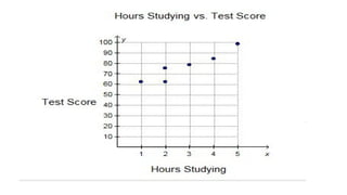
49. Practical Example: Hours Studied vs. Test Scores
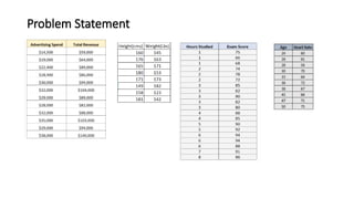
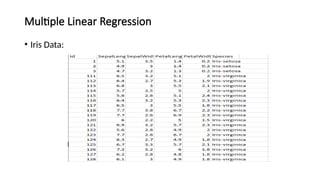
• Data:
Example dataset with hours studied and corresponding test scores.
• Hours studied: [1, 2, 3, 4, 5]
• Test scores: [50, 55, 60, 65, 70]
• Regression Line:
After performing linear regression, we get the equation for the line:
• Test Score= 50 + 5 (Hours Studied)
⋅
• This means that for every additional hour of study, the score increases by 5 points.

50. Advantages of Linear Regression
• Simple and Easy to Understand:
The model is easy to explain and interpret, making it a good starting
point for prediction.
• Quick Computation:
Linear regression can be computed quickly, even with large datasets.
• Clear Interpretation:
The coefficients (β0 and β1​
) are easy to understand in practical terms.

51. Limitations of Linear Regression
• Assumes a Linear Relationship:
It only works well if the relationship between the variables is linear. If
the relationship is non-linear, this method may not work.
• Sensitive to Outliers:
Outliers (data points far from the line) can greatly affect the line.

52. Applications of Linear Regression
• Predicting Sales:
Estimating sales based on advertising budget or marketing spend.
• Predicting Growth:
Estimating population growth or economic trends based on certain
factors.
• Medical Research:
Predicting the impact of various factors (e.g., age, lifestyle) on health
outcomes.
• Real Estate:
Estimating house prices based on factors like square footage, number
of rooms, and location.

53. Conclusion
• Linear regression is a powerful, simple, and widely used tool for
making predictions.
• It’s most useful when there is a linear relationship between the
independent and dependent variables.
• Understanding its basic principles, like the slope and intercept, helps
in applying linear regression effectively.

54. STA6166-RegBasics 55
Relationships
In science, we frequently measure two or more variables on the same
individual (case, object, etc). We do this to explore the nature of the
relationship among these variables. There are two basic types of
relationships.
• Cause-and-effect relationships.
• Functional relationships.
Function: a mathematical relationship enabling us to predict what
values of one variable (Y) correspond to given values of another
variable (X).
• Y: is referred to as the dependent variable, the response
variable or the predicted variable.
• X: is referred to as the independent variable, the explanatory
variable or the predictor variable.
What is Regression?

55. STA6166-RegBasics 57
b0: intercept,
b1: linear coefficient,
b2: quadratic coefficient.
2
2
1
0 X
b
X
b
b
Y 


Example: Polynomial relationship (e.g.
Y=crop yield vs. X=pH)