Statistics

1. Simple Linear Regression
Simple Linear Regression

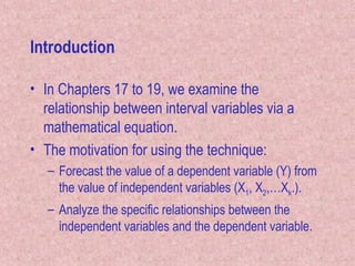
2. Introduction
• In Chapters 17 to 19, we examine the
relationship between interval variables via a
mathematical equation.
• The motivation for using the technique:
– Forecast the value of a dependent variable (Y) from
the value of independent variables (X1, X2,…Xk.).
– Analyze the specific relationships between the
independent variables and the dependent variable.

3. House size
House
Cost
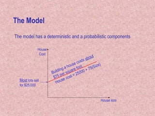
Most lots sell
for $25,000
Building a house costs about
$75 per square foot.
House cost = 25000 + 75(Size)
The Model
The model has a deterministic and a probabilistic components

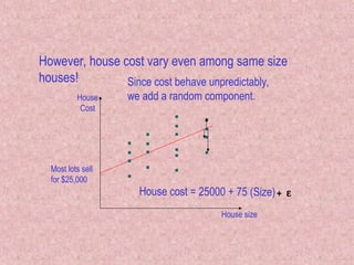
4. House cost = 25000 + 75 (Size)
House size
House
Cost
Most lots sell
for $25,000

However, house cost vary even among same size
houses! Since cost behave unpredictably,
we add a random component.

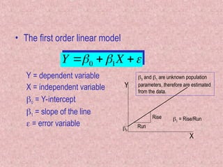
5. • The first order linear model
Y = dependent variable
X = independent variable
0 = Y-intercept
1 = slope of the line
 = error variable

Y 0  1X 
X
Y
0
Run
Rise  = Rise/Run
0 and 1 are unknown population
parameters, therefore are estimated
from the data.

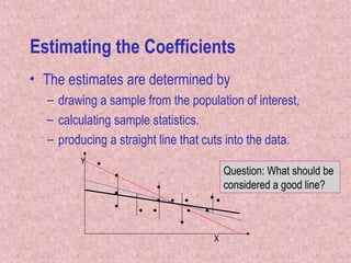
6. Estimating the Coefficients
• The estimates are determined by
– drawing a sample from the population of interest,
– calculating sample statistics.
– producing a straight line that cuts into the data.










Question: What should be
considered a good line?
X
Y

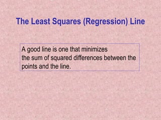
7. The Least Squares (Regression) Line
A good line is one that minimizes
the sum of squared differences between the
points and the line.

8. 3
3




4
1
1
4
(1,2)
2
2
(2,4)
(3,1.5)
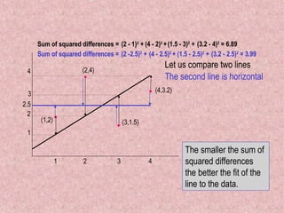
Sum of squared differences = (2 - 1)2
+ (4 - 2)2
+(1.5 - 3)2
+
(4,3.2)
(3.2 - 4)2
= 6.89
Sum of squared differences = (2 -2.5)2
+ (4 - 2.5)2
+ (1.5 - 2.5)2
+ (3.2 - 2.5)2
= 3.99
2.5
Let us compare two lines
The second line is horizontal
The smaller the sum of
squared differences
the better the fit of the
line to the data.

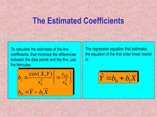
9. The Estimated Coefficients
To calculate the estimates of the line
coefficients, that minimize the differences
between the data points and the line, use
the formulas:
b1 
cov(X,Y)
sX
2 
sXY
sX
2






b0 Y  b1 X
The regression equation that estimates
the equation of the first order linear model
is:

ˆ
Y b0  b1X

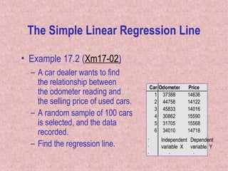
10. • Example 17.2 (Xm17-02)
– A car dealer wants to find
the relationship between
the odometer reading and
the selling price of used cars.
– A random sample of 100 cars
is selected, and the data
recorded.
– Find the regression line.
Car Odometer Price
1 37388 14636
2 44758 14122
3 45833 14016
4 30862 15590
5 31705 15568
6 34010 14718
. . .
. . .
. . .
Independent
variable X
Dependent
variable Y
The Simple Linear Regression Line

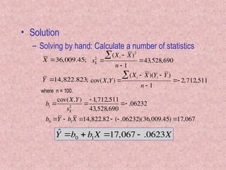
11. • Solution
– Solving by hand: Calculate a number of statistics

X 36,009.45;
Y 14,822.823;

sX
2

(Xi  X)2

n  1
43,528,690
cov(X,Y) 
(Xi  X)(Yi  Y )

n  1
 2,712,511
where n = 100.

b1 
cov(X,Y)
sX
2

 1,712,511
43,528,690
 .06232
b0 Y  b1X 14,822.82  ( .06232)(36,009.45) 17,067
ˆ
Y b0  b1X 17,067  .0623X

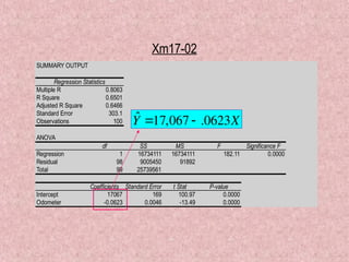
12. • Solution – continued
– Using the computer (Xm17-02)
Tools > Data Analysis > Regression >
[Shade the Y range and the X range] > OK

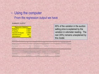
13. SUMMARY OUTPUT
Regression Statistics
Multiple R 0.8063
R Square 0.6501
Adjusted R Square 0.6466
Standard Error 303.1
Observations 100
ANOVA
df SS MS F Significance F
Regression 1 16734111 16734111 182.11 0.0000
Residual 98 9005450 91892
Total 99 25739561
Coefficients Standard Error t Stat P-value
Intercept 17067 169 100.97 0.0000
Odometer -0.0623 0.0046 -13.49 0.0000

ˆ
Y 17,067  .0623X
Xm17-02

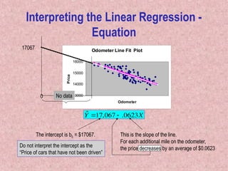
14. This is the slope of the line.
For each additional mile on the odometer,
the price decreases by an average of $0.0623
Odometer Line Fit Plot
13000
14000
15000
16000
Odometer
Price

ˆ
Y 17,067  .0623X
Interpreting the Linear Regression -
Equation
The intercept is b0 = $17067.
0 No data
Do not interpret the intercept as the
“Price of cars that have not been driven”
17067

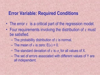
15. Error Variable: Required Conditions
• The error is a critical part of the regression model.
• Four requirements involving the distribution of  must
be satisfied.
– The probability distribution of  is normal.
– The mean of  is zero: E() = 0.
– The standard deviation of  is  for all values of X.
– The set of errors associated with different values of Y are
all independent.

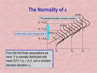
16. The Normality of 
From the first three assumptions we
have: Y is normally distributed with
mean E(Y) = 0 + 1X, and a constant
standard deviation 

0 + 1X1
0 + 1 X2
0 + 1 X3
E(Y|X2)
E(Y|X3)
X1 X2 X3

E(Y|X1)

The standard deviation remains constant,
but the mean value changes with X

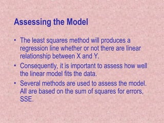
17. Assessing the Model
• The least squares method will produces a
regression line whether or not there are linear
relationship between X and Y.
• Consequently, it is important to assess how well
the linear model fits the data.
• Several methods are used to assess the model.
All are based on the sum of squares for errors,
SSE.

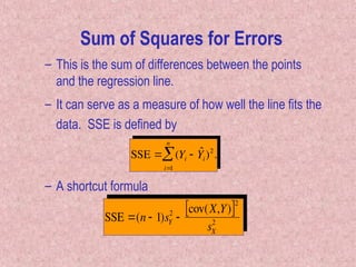
18. – This is the sum of differences between the points
and the regression line.
– It can serve as a measure of how well the line fits the
data. SSE is defined by

SSE  (Yi  ˆ
Yi)2
i
1
n
 .
Sum of Squares for Errors
SSE (n  1)sY
2

cov(X,Y)
 2
sX
2
– A shortcut formula

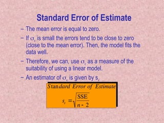
19. – The mean error is equal to zero.
– If  is small the errors tend to be close to zero
(close to the mean error). Then, the model fits the
data well.
– Therefore, we can, use  as a measure of the
suitability of using a linear model.
– An estimator of  is given by s
Standard Error of Estimate
s 
SSE
n  2
Standard Error of Estimate

20. • Example 17.3
– Calculate the standard error of estimate for Example 17.2,
and describe what does it tell you about the model fit?
• Solution
13
.
303
98
450
,
005
,
9
2
SSE
450
,
005
,
9
690
,
528
,
43
)
511
,
712
,
2
(
)
996
,
259
(
99
)]
,
[cov(
)
1
(
SSE
996
,
259
1
)
ˆ
(
2
2
2
2
2
2
















n
s
s
Y
X
s
n
n
Y
Y
s
X
Y
i
i
Y

Calculated before
It is hard to assess the model based
on s even when compared with the
mean value of Y.
823
,
14
y
1
.
303
s 



21. 















 




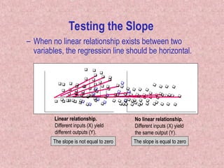
Testing the Slope
– When no linear relationship exists between two
variables, the regression line should be horizontal.



















































 









 


























Different inputs (X) yield
different outputs (Y).
No linear relationship.
Different inputs (X) yield
the same output (Y).
The slope is not equal to zero The slope is equal to zero
Linear relationship.
Linear relationship.
Linear relationship.
Linear relationship.

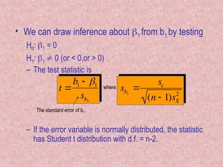
22. • We can draw inference about 1 from b1 by testing
H0: 1 = 0
H1: 1  0 (or < 0,or > 0)
– The test statistic is
– If the error variable is normally distributed, the statistic
has Student t distribution with d.f. = n-2.

t 
b1  1
sb1
The standard error of b1.

sb1

s
(n  1)sX
2
where

23. • Example 17.4
– Test to determine whether there is enough evidence
to infer that there is a linear relationship between the
car auction price and the odometer reading for all
three-year-old Tauruses, in Example 17.2.
Use  = 5%.

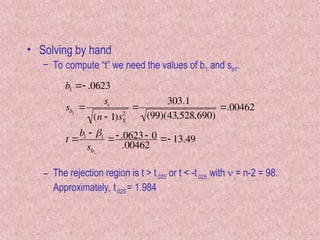
24. • Solving by hand
– To compute “t” we need the values of b1 and sb1.
– The rejection region is t > t.025 or t < -t.025 with  = n-2 = 98.
Approximately, t.025 = 1.984

b1  .0623
sb1

s
(n  1)sX
2

303.1
(99)(43,528,690)
.00462
t 
b1  1
sb1
 .0623 0
.00462
 13.49

25. Price Odometer SUMMARY OUTPUT
14636 37388
14122 44758 Regression Statistics
14016 45833 Multiple R 0.8063
15590 30862 R Square 0.6501
15568 31705 Adjusted R Square 0.6466
14718 34010 Standard Error 303.1
14470 45854 Observations 100
15690 19057
15072 40149 ANOVA
14802 40237 df SS MS F Significance F
15190 32359 Regression 1 16734111 16734111 182.11 0.0000
14660 43533 Residual 98 9005450 91892
15612 32744 Total 99 25739561
15610 34470
14634 37720 Coefficients Standard Error t Stat P-value
14632 41350 Intercept 17067 169 100.97 0.0000
15740 24469 Odometer -0.0623 0.0046 -13.49 0.0000
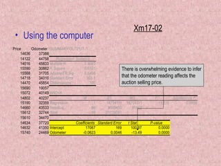
• Using the computer
There is overwhelming evidence to infer
that the odometer reading affects the
auction selling price.
Xm17-02

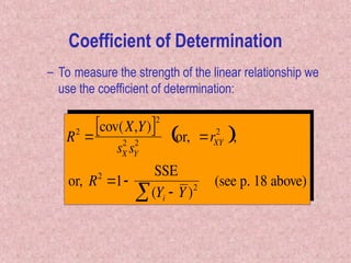
26. – To measure the strength of the linear relationship we
use the coefficient of determination:
R2

cov(X,Y)
 2
sX
2
sY
2 or, rXY
2
 ;
or, R2
1
SSE
(Yi  Y )2

(see p. 18 above)
Coefficient of Determination

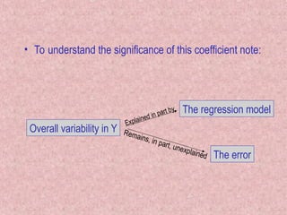
27. • To understand the significance of this coefficient note:
Overall variability in Y
The regression model
Remains, in part, unexplained The error
Explained in part by

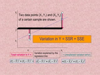
28. x1 x2
y1
y2
y
Two data points (X1,Y1) and (X2,Y2)
of a certain sample are shown.

(Y1  Y )2
 (Y2  Y )2


( ˆ
Y1  Y )2
 ( ˆ
Y2  Y )2

(Y1  ˆ
Y1)2
 (Y2  ˆ
Y2)2
Total variation in Y =
Variation explained by the
regression line
+ Unexplained variation (error)
Variation in Y = SSR + SSE

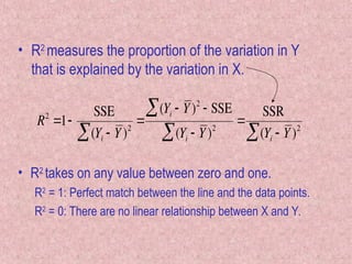
29. • R2
measures the proportion of the variation in Y
that is explained by the variation in X.

R2
1
SSE
(Yi  Y)2


(Yi  Y)2
  SSE
(Yi  Y)2


SSR
(Yi  Y)2

• R2
takes on any value between zero and one.
R2
= 1: Perfect match between the line and the data points.
R2
= 0: There are no linear relationship between X and Y.

30. • Example 17.5
– Find the coefficient of determination for Example 17.2;
what does this statistic tell you about the model?
• Solution
– Solving by hand;

R2

[cov(X,Y)]2
sX
2
sY
2
 [ 2,712,511]2
(43,528,688)(259,996) .6501

31. SUMMARY OUTPUT
Regression Statistics
Multiple R 0.8063
R Square 0.6501
Adjusted R Square 0.6466
Standard Error 303.1
Observations 100
ANOVA
df SS MS F Significance F
Regression 1 16734111 16734111 182.11 0.0000
Residual 98 9005450 91892
Total 99 25739561
CoefficientsStandard Error t Stat P-value
Intercept 17067 169 100.97 0.0000
Odometer -0.0623 0.0046 -13.49 0.0000
– Using the computer
From the regression output we have
65% of the variation in the auction
selling price is explained by the
variation in odometer reading. The
rest (35%) remains unexplained by
this model.