Hypothesis testing

HYPOTHESIS TESTING
Dr. Perini PraveenaSri
Associate Professor
Atria Institute of Technology

HYPOTHESIS TESTING
A hypothesis is a tentative statement about the relationship between two or
more variables. It is a specific, testable prediction about what you expect to
happen in a study.
For example, a study designed to look at the relationship between sleep deprivation
and test performance. This might have a hypothesis that states, "This study is
designed to assess the hypothesis that sleep-deprived people will perform worse on
a test than individuals who are not sleep deprived.“
Descriptive Statistics and Inferential statistics are two major categories of statistical
procedures. For Inferential Statistics ,the first , estimation of population values, was
used with sampling .The second, was testing statistical hypotheses, is the
primary subject.

How Is a Hypothesis Used in the Scientific Method of Economic Model ?
 The scientific research method in social sciences involves the
following steps:
1. Forming a question
2. Performing background research
3. Creating a hypothesis
4. Designing an experiment
5. Collecting data
6. Analyzing the results
7. Drawing conclusions
8. Communicating the results with policy recommendations

Process of Hypothesis
The hypothesis is what the researchers' predict the relationship between
two or more variables, but it involves more than a guess. It should be a
professional guess.
Most of the time, the hypothesis begins with a question which is then
explored through background research. It is only at this point that
researchers begin to develop a testable hypothesis.
In a study exploring the effects of a water scarcity , the hypothesis
might be that researchers expect the water scarcity to have some type
of effect on the production of electricity . In Energy Economics, the
hypothesis might focus on how a certain aspect of the water shortages
has impounding risks on the production of electricity.

 Unless you are creating a study that is exploratory in nature, your
hypothesis should always explain what you expect to happen during
the course of your experiment or research.
 Remember, a hypothesis does have to be correct or may not be. The
hypothesis can be accepted or rejected. While the hypothesis predicts
what the researchers expect to see, the goal of the research is to determine
whether this guess is right or wrong. The guess should be a professional
guess with backing of pilot survey approach.
 When conducting an experiment, researchers might explore a number of
factors to determine which ones might contribute to the ultimate outcome.
 In many cases, researchers may find that the results of an experiment do
not support the original hypothesis. When writing up these results, the
researchers might suggest other options that should be explored in
future studies.

CHARACTERISTICS OF HYPOTHESIS: HYPOTHESIS MUST
POSSESS THE FOLLOWING CHARACTERISTICS:
 (i) Hypothesis should be clear and precise. If the hypothesis is not clear and
precise, the inferences drawn on its basis cannot be taken as reliable.
 (ii) Hypothesis should be capable of being tested. In a swamp of untestable
hypotheses, many a time the research programmes have bogged down.
 (iii) Some prior study may be done by researcher in order to make hypothesis a
testable one. A hypothesis “is testable if other deductions can be made from
it which, in turn, can be confirmed or disproved by observation.”
 (iii) Hypothesis should state relationship between variables, if it happens to be a
relational hypothesis.
 (iv) Hypothesis should be limited in scope and must be specific. A researcher
must remember that narrower hypotheses are generally more testable and he
should develop such hypotheses.

 (v)Hypothesis should be stated as far as possible in most simple terms so
that the same is easily understandable by all concerned. But one must
remember that simplicity of hypothesis has nothing to do with its
significance.
(vi) Hypothesis should be consistent with most known facts i.e., it
must be consistent with a substantial body of established facts. In other
words, it should be one which judges accept as being the most likely.
(vii) Hypothesis should be amenable to testing within a reasonable
time. One should not use even an excellent hypothesis, if the same cannot
be tested in reasonable time for one cannot spend a life-time collecting
data to test it.

(viii) Hypothesis must explain the facts that gave rise
to the need for explanation.
This means that by using the hypothesis plus other
known and accepted generalizations (universality ) ,
one should be able to deduce the original problem
condition.
Thus hypothesis must actually explain what it claims to
explain; it should have empirical reference.

BASICS OF HYPOTHESIS : ASSESSMENT OF STATISTICAL SIGNIFICANCE : AN
HYPOTHETICAL EXPERIMENT
Hypothesis testing is guided by statistical analysis.
Statistical significance is calculated using a p-value, which tells you
the probability of your result being observed, given that a certain
statement (the null hypothesis) is true.
If this p-value is less than the significance level set (usually
0.05), the experimenter can assume that the null hypothesis is
false and accept the alternative hypothesis.
Using a simple t-test, you can calculate a p-value and determine
significance between two different groups of a dataset.

SETTING AN EXPERIMENT FOR HYPOTHESIS TESTING
1.Define your hypotheses.
The first step in assessing statistical significance is defining the question you want to answer and
stating your hypothesis. The hypothesis is a statement about your experimental data and the
differences that may be occurring in the population. For any experiment, there is both a null and
an alternative hypothesis. Generally, you will be comparing two groups to see if they are the same or
different.
The null hypothesis (H0) generally states that there is no difference between
your two data sets. For example: Students who read the material before class do
not get better final grades.
The alternative hypothesis (Ha) is the opposite of the null hypothesis and is
the statement you are trying to support with your experimental data. For
example: Students who read the material before class do get better final
grades.

2 Set the significance level to determine how unusual your
data must be before it can be considered significant.
The significance level (also called alpha) is the threshold that you set to determine
significance. If your p-value is less than or equal to the set significance level,
the data is considered statistically significant.
As a general rule, the significance level (or alpha) is commonly set to 0.05, meaning
that the probability of observing the differences seen in your data by chance is
just 5%.
A higher confidence level (and, thus, a lower p-value) means the results are more
significant.
If you want higher confidence in your data, set the p-value lower to 0.01. Lower p-
values are generally used in manufacturing when detecting flaws in products.
It is very important to have high confidence that every part will work exactly as it is

3 Decide to use a one-tailed or two-tailed test.
One of the assumptions a t-test makes is that your data is distributed normally. A normal
distribution of data forms a bell curve with the majority of the samples falling in the middle.
The t-test is a mathematical test to see if your data falls outside of the normal distribution, either
above or below, in the “tails” of the curve.
A one-tailed test is more powerful than a two-tailed test, as it examines the
potential of a relationship in a single direction (such as above the control group),
while a two-tailed test examines the potential of a relationship in both directions
(such as either above or below the control group).
If you are not sure if your data will be above or below the control group, use a two-
tailed test. This allows you to test for significance in either direction.
If you know which direction you are expecting your data to trend towards, use a one-
tailed test. In the given example, you expect the student’s grades to improve;
therefore, you will use a one-tailed test.

4 Determine sample size with a power analysis.
The power of a test is the probability of observing the expected result,
given a specific sample size. The common threshold for power (or β) is 80%.
A power analysis can be a bit tricky without some preliminary data, as you need some
information about your expected means between each group and their
standard deviations. Use a power analysis calculator online to determine the
optimal sample size for your data.
Researchers usually do a small pilot study to inform their power analysis and
determine the sample size needed for a larger, comprehensive study.
If you do not have the means to do a complex pilot study, make some estimations
about possible means based on reading the literature and studies that other
individuals may have performed. This will give you a good place to start for
sample size.

Calculating the Standard Deviation
1 Define the formula for standard deviation. The standard deviation is a measure of how
spread out your data is. It gives you information on how similar each data point is within
your sample, which helps you determine if the data is significant.
At first glance, the equation may seem a bit complicated, but these steps will walk you through the
process of the calculation.
The formula is s = √∑((xi – µ)2/(N – 1)).
s is the standard deviation.
∑ indicates that you will sum all of the sample values collected.
xi represents each individual value from your data.
µ is the average (or mean) of your data for each group.
N is the total sample number.

2 Average the samples in each group.
To calculate the standard deviation, first you must take the average of the
samples in the individual groups. The average is designated with the
Greek letter mu or µ. To do this, simply add each sample together and
then divide by the total number of samples.
For example, to find the average grade of the group that read the
material before class, let’s look at some data.
For simplicity, we will use a dataset of 5 points: 90, 91, 85, 83, and 94.
Add all the samples together: 90 + 91 + 85 + 83 + 94 = 443.
Divide the sum by the sample number, N = 5: 443/5 = 88.6.
The average grade for this group is 88.6.

3Subtract each sample from the average.
The next part of the calculation involves the (xi – µ) portion of the equation. You
will subtract each sample from the average just calculated.
For our example you will end up with five subtractions.(90 – 88.6), (91- 88.6), (85
– 88.6), (83 – 88.6), and (94 – 88.6).
The calculated numbers are now 1.4, 2.4, -3.6, -5.6, and 5.4.
4 Square each of these numbers and add them together.
Each of the new numbers you have just calculated will now be squared. This step
will also take care of any negative signs.
If you have a negative sign after this step or at the end of your calculation, you
may have forgotten this step. In our example, we are now working with 1.96, 5.76,
12.96, 31.36, and 29.16.
Summing these squares together yields: 1.96 + 5.76 + 12.96 + 31.36 + 29.16 =

5 Divide by the total sample number minus 1.
The formula divides by N – 1 because it is correcting for the fact that you haven’t counted an
entire population; you are taking a sample of the population of all students to make an
estimation.
Subtract: N – 1 = 5 – 1 = 4
Divide: 81.2/4 = 20.3
6 Take the square root.
Once you have divided by the sample number minus one, take the square root of this
final number.
This is the last step in calculating the standard deviation. There are statistical
programs that will do this calculation for you after inputting the raw data.
For our example, the standard deviation of the final grades of students who read
before class is: s =√20.3 = 4.51.

Determining Significance
1Calculate the variance between your 2 sample groups.
Up to this point, the example has only dealt with 1 of the sample groups. If you are
trying to compare 2 groups, you will obviously have data from both.
Calculate the standard deviation of the second group of samples and use that to
calculate the variance between the 2 experimental groups.
The formula for variance is sd = √((s1/N1) + (s2/N2)).
sd is the variance between your groups.
s1 is the standard deviation of group 1 and N1 is the sample size of group 1.
s2 is the standard deviation of group 2 and N2 is the sample size of group 2.
For our example, let’s say the data from group 2 (students who didn’t read before
class) had a sample size of 5 and a standard deviation of 5.81. The variance is:
sd = √((s1)2/N1) + ((s2)2/N2))
sd = √(((4.51)2/5) + ((5.81)2/5)) = √((20.34/5) + (33.76/5)) = √(4.07 + 6.75) = √10.82 =

2 Calculate the t-score of your data.
A t-score allows you to convert your data into a form that allows you to compare it to other
data.
T-scores allow you to perform a t-test that lets you calculate the probability of two groups
being significantly different from each other. The formula for a t-score is: t = (µ1 – µ2)/sd.
µ1 is the average of the first group.
µ2 is the average of the second group.
sd is the variance between your samples.
Use the larger average as µ1 so you will not have a negative t-value.
For our example, let’s say the sample average for group 2 (those who didn’t read) was 80.
The t-score is: t = (µ1 – µ2)/sd = (88.6 – 80)/3.29 = 2.61.

3 Determine the degrees of freedom of your sample.
When using the t-score, the number of degrees of freedom is determined using
the sample size. Add up the number of samples from each group and then
subtract two. For our example, the degrees of freedom (d.f.) are 8 because
there are five samples in the first group and five samples in the second
group ((5 + 5) – 2 = 8)
The number of degrees of freedom generally refers to the number of
independent observations in a sample minus the number of population
parameters that must be estimated from sample data. For example, the exact
shape of a t distribution is determined by its degrees of freedom.

4 Use a t table to evaluate significance.
A table of t-scores and degrees of freedom can be found in a
standard statistics book or online. Look at the row containing the
degrees of freedom for your data and find the p-value that
corresponds to your t-score.
With 8 d.f. and a t-score of 2.61, the p-value for a one-tailed
test falls between 0.01 and 0.025. Because we set our
significance level less than or equal to 0.05, our data is
statistically significant. With this data, we reject the null
hypothesis and accept the alternative hypothesis: students
who read the material before class get better final grades.

5 Consider a follow up study.
Many researchers do a small pilot study with a few measurements to help them
understand how to design a larger study.
Doing another study, with more measurements, will help increase your confidence about
your conclusion.
A follow-up study can help you determine if any of your
conclusions contained
type I error (observing a difference when there isn’t one,
or false rejection of the null hypothesis)
or type II error (failure to observe a difference when
there is one, or false acceptance of the null hypothesis).

Tests for statistical significance are used to estimate the probability that a relationship observed in the data
occurred only by chance; the probability that the variables are really unrelated in the population.
To determine whether a result is statistically significant, a researcher calculates a p-value, which is the
probability of observing an effect of the same magnitude or more extreme given that the null hypothesis is
true.
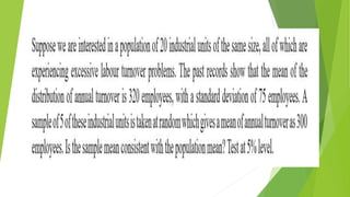
Statistical hypothesis testing is used to determine whether the result of a data set is statistically significant.
This test provides a p-value, representing the probability that random chance could explain the result. In general, a
p-value of 5% or lower is considered to be statistically significant.
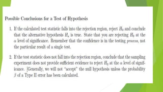
The 7 Step Process of Statistical Hypothesis Testing
Step 1: State the Null Hypothesis. ...
Step 2: State the Alternative Hypothesis. ...
Step 3: Set [Math Processing Error] ...
Step 4: Collect Data. ...
Step 5: Calculate a test statistic. ...
Step 6: Construct rejection regions. ...
Step 7: Based on steps 5 and 6, draw a conclusion about H0

Logic of Hypothesis Testing
 In classical tests of significance, two kinds of hypotheses are used. The null hypothesis
(H0) is used for testing. It is a statement that no difference exists between the
parameter (a measure taken by a census of the population or a prior measurement
of a sample of the population) and the statistic being compared to it (a measure
from a recently drawn sample of the population).
 Analysts usually test to determine whether there has been no change in the
population of interest or whether a real difference exists.
 Why not state the hypothesis in a positive form? Why not state that any difference
between the sample statistic and the population parameter is due to some reason?
 Unfortunately, this type of hypothesis cannot be tested definitively.
 Evidence that is consistent with a hypothesis stated in a positive form can almost never
be taken as conclusive grounds for accepting the hypothesis. A finding that is consistent
with this type of hypothesis might be consistent with other hypotheses too, and thus it
does not demonstrate the truth of the given hypothesis.

EXAMPLES FOR LOGIC OF TESTING HYPOTHESIS
For example 1, suppose a coin is suspected of being biased in favor of heads. The
coin is flipped 100 times and the outcome is 52 heads. It would not be correct to jump
to the conclusion that the coin is biased simply because more than the expected
number of 50 heads resulted.
The reason is that 52 heads is consistent with the hypothesis that the coin is fair. On
the other hand, flipping 85 or 90 heads in 100 flips would seem to contradict the
hypothesis of a fair coin. In this case there would be a strong case for a biased coin.

TESTS OF HYPOTHESIS
Suppose you wanted to determine whether the mean level of a driver's
blood alcohol exceeds the legal limit after two drinks,
or whether the majority of registered voters approve of the president's
performance.
In both cases, you are interested in making an inference about how the
value of a parameter relates to a specified numerical value. Is it
less than, equal to, or greater than the specified number? This type
of inference, called a test of hypothesis.

The Elements of a Test of Hypothesis
The elements of the test:
1. Null hypothesis(H0): A theory about the values of one or more
population parameters. The theory generally represents the
status quo, which we adopt until it is proven false.
By convention, the theory is stated as H0: parameter=value.
2. Alternative (research) hypothesis (Ha): A theory that contradicts
the null hypothesis. The theory generally represents that which
we will accept only when sufficient evidence exist to establish its
truth.
3. Test statistic: A sample statistic used to decide whether to reject
the null hypothesis.

4. Rejection region: The numerical values of the test statistic for which
the null hypothesis will be rejected.
The rejection region is chosen so that the probability is that it will
contain the test statistic when the null hypothesis is true, thereby
leading to a Type I error.
The value of is usually chosen to be small (e.g, 0.01, 0.05, or 0.10) and
is referred to as the level of significance of the test.
5. Assumptions: Clear statements of any assumptions made about
the population(s) being sampled.
6. Experiment and calculation of test statistic: Performance of the
sampling experiment and determination of the numerical value of
the test statistic.

7. Conclusion:
a. If the numerical value of the test statistic falls into the rejection region,
we reject the null hypothesis and conclude that the alternative hypothesis
is true. We know that the hypothesis-testing process will lead to this
conclusion incorrectly (a Type I error) only 100% of the time when H0 is
true.or unnecessarily falsifying null hypothesis that is true.
b. If the test statistic does not fall into the rejection region, we do not
reject H0. Thus, we reserve judgement about which hypothesis is true.
We do not conclude that the null hypothesis is true because we do not (in
general) know the probability
that our test procedure will lead to an incorrect acceptance of H0 (a Type
II error).

Large-Sample Test of Hypothesis about a Population Mean
The null and alternative hypotheses may take one of several forms, a
one-tailed( or one- sided) statistical test and a two-tailed (or two-sided)
hypothesis.
Steps for Selecting the Null the Alternative Hypotheses
1. Select the alternative hypothesis as that which the sampling
experiment is intended to establish. The alternative hypothesis will
assume on of three forms:

EXEMPLARY ILLUSTRATIONS OF HYPOTHESIS TESTING
 For example 2, Honda, Toyota, Chrysler, Nissan, Ford, and other auto companies produce hybrid vehicles
using an advanced technology that combines a small gas engine with an electric motor. The vehicles
run on an electric motor at slow speeds but shift to both the gasoline motor and the electric motor at city and
higher freeway speeds. Their advertising strategies focus on fuel economy.
 Let’s say that the hybrid Toyota has maintained an average of about 60 miles per
gallon (mpg) with a standard deviation of 10 mpg. Suppose researchers discover
by analyzing all production vehicles that the mpg is now 61. Is this difference
statistically significant from 60?
 Of course it is, because the difference is based on a census of the vehicles and
there is no sampling involved. It has been demonstrated conclusively that the
population average has moved from 60 to 61 mpg. Although it is of statistical
significance, whether it is of practical significance is another question.
 If a decision maker judges that this variation has no real importance, then it is of
little practical significance.

Since it would be too expensive to analyze all of a manufacturer’s vehicles frequently,
we resort to sampling.
Assume a sample of 25 cars is randomly selected and the average mpg is calculated
to be 64. Is this statistically significant? The answer is not obvious. It is significant if
there is good reason to believe the average mpg of the total population has moved
up from 60.
Since the evidence consists of only a sample, consider the second possibility: that
this is only a random sampling error and thus is not significant.
The task is to decide whether such a result from this sample is or is not statistically
significant. To answer this question, one needs to consider further the logic of
hypothesis testing.

ALTERNATIVE HYPOTHESES: TWO-TAILED AND ONE-TAILED TESTS.
A two-tailed test, or nondirectional test, considers two
possibilities: the average could be more than 60 mpg, or
it could be less than 60.
To test this hypothesis, the regions of rejection are
divided into two tails of the distribution. A one-tailed
test, or directional test, places the entire probability of
an unlikely outcome into the tail specified by the
alternative hypothesis.

In Exhibit 17-2, the first diagram represents a nondirectional hypothesis, and the second
is a directional hypothesis of the “greater than” variety.

If we reject a null hypothesis (finding a statistically significant difference), then we are accepting the
alternative hypothesis. In either accepting or rejecting a null hypothesis, we can make incorrect
decisions.
A null hypothesis can be accepted when it should have been rejected or rejected when it should have

EXAMPLE 3: AN ANALOGY TO THE AMERICAN LEGAL SYSTEM.
 In our system of justice, the innocence of an indicted person is presumed until
proof of guilt beyond a reasonable doubt can be established. In hypothesis
testing, this is the null hypothesis;
 There should be no difference between the presumption of innocence and the
outcome unless contrary evidence is furnished. Once evidence establishes beyond
reasonable doubt that innocence can no longer be maintained, a just conviction is
required. This is equivalent to rejecting the null hypothesis and accepting the
alternative hypothesis.
 Incorrect decisions or errors are the other two possible outcomes. We can unjustly
convict an innocent person, or we can acquit a guilty person.

Example 4:
 A recent study estimated that 20% of all college students in the United States smoke. The head of Health
Services at Goodheart University (GU) suspects that the proportion of smokers may be lower at GU. In hopes of
confirming her claim, the head of Health Services chooses a random sample of 400 Goodheart students, and
finds that 70 of them are smokers.
 Let’s analyze this example using the 4 steps outlined above:
1. Stating the claims: There are two claims here:
 Claim 1: The proportion of smokers at Goodheart is 0.20.
 Claim 2: The proportion of smokers at Goodheart is less than 0.20.
Claim 1 basically says “nothing special goes on at Goodheart University; the proportion of smokers there is no
different from the proportion in the entire country.” This claim is challenged by the head of Health Services,
who suspects that the proportion of smokers at Goodheart is lower.
2. Choosing a sample and collecting data: A sample of n = 400 was chosen, and summarizing the data revealed that the
sample proportion of smokers is p-hat = 70/400 = 0.175.While it is true that 0.175 is less than 0.20, it is not clear whether
this is strong enough evidence against claim 1. We must account for sampling variation.

3 Assessment of evidence: In order to assess whether the data provide strong enough evidence against claim
1, we need to ask ourselves: How surprising is it to get a sample proportion as low as p-hat = 0.175 (or
lower), assuming claim 1 is true?
In other words, we need to find how likely it is that in a random sample of size n = 400 taken from a
population where the proportion of smokers is p = 0.20 we’ll get a sample proportion as low as p-hat = 0.175
(or lower).
It turns out that the probability that we’ll get a sample proportion as low as p-hat = 0.175 (or lower) in such a
sample is roughly 0.106 (do not worry about how this was calculated at this point – however, if you think
about it hopefully you can see that the key is the sampling distribution of p-hat).
4 .Conclusion: Well, we found that if claim 1 were true there is a probability of 0.106 of observing data like
that observed or more extreme.
Now you have to decide …Do you think that a probability of 0.106 makes our data rare enough (surprising
enough) under claim 1 so that the fact that we did observe it is enough evidence to reject claim 1? Or do
you feel that a probability of 0.106 means that data like we observed are not very likely when claim 1 is true,
but they are not unlikely enough to conclude that getting such data is sufficient evidence to reject claim 1.
Basically, this is your decision. However, it would be nice to have some kind of guideline about what is
generally considered surprising enough.

EXAMPLE 5:
A certain prescription allergy medicine is supposed to contain an average of 245 parts per
million (ppm) of a certain chemical. If the concentration is higher than 245 ppm, the drug will
likely cause unpleasant side effects, and if the concentration is below 245 ppm, the drug may
be ineffective. The manufacturer wants to check whether the mean concentration in a large
shipment is the required 245 ppm or not.
To this end, a random sample of 64 portions from the large shipment is tested, and it is found
that the sample mean concentration is 250 ppm with a sample standard deviation of 12 pp
m.
1.Stating the claims:
Claim 1: The mean concentration in the shipment is the required 245 ppm.
Claim 2: The mean concentration in the shipment is not the required 245 ppm.
Note that again, claim 1 basically says: “There is nothing unusual about this shipment, the
mean concentration is the required 245 ppm.” This claim is challenged by the manufacturer,
who wants to check whether that is, indeed, the case or not.

2. Choosing a sample and collecting data: A sample of n = 64 portions is chosen and after
summarizing the data it is found that the sample mean concentration is x-bar = 250 and the sample
standard deviation is s = 12.
Is the fact that x-bar = 250 is different from 245 strong enough evidence to reject claim 1 and conclude
that the mean concentration in the whole shipment is not the required 245? In other words, do the
data provide strong enough evidence to reject claim 1?
3. Assessing the evidence: In order to assess whether the data provide strong enough evidence
against claim 1, we need to ask ourselves the following question: If the mean concentration in the
whole shipment were really the required 245 ppm (i.e., if claim 1 were true), how surprising would it be
to observe a sample of 64 portions where the sample mean concentration is off by 5 ppm or more (as
we did)?
It turns out that it would be extremely unlikely to get such a result if the mean concentration were
really the required 245. There is only a probability of 0.0007 (i.e., 7 in 10,000) of that happening. (Do
not worry about how this was calculated at this point, but again, the key will be the sampling
distribution.)

4. Making conclusions: Here, it is pretty clear that a sample like the one we observed or more
extreme is VERY rare (or extremely unlikely) if the mean concentration in the shipment were
really the required 245 ppm.
The fact that we did observe such a sample therefore provides strong evidence against claim 1,
so we reject it and conclude with very little doubt that the mean concentration in the shipment is
not the required 245 ppm.

Example:6
 Is there a relationship between gender and combined scores (Math + Verbal) on the SAT exam?
Following a report on the College Board website, which showed that in 2003, males scored generally higher than
females on the SAT exam, an educational researcher wanted to check whether this was also the case in her
school district. The researcher chose random samples of 150 males and 150 females from her school district,
collected data on their SAT performance and found the following:
Females
n mean standard deviation
150 1010 206
Males n mean standard deviation
150 1025 212

Again, let’s see how the process of hypothesis testing works for this example:
1. Stating the claims:
Claim 1: Performance on the SAT is not related to gender (males and females score the same).
Claim 2: Performance on the SAT is related to gender – males score higher.
Note that again, claim 1 basically says: “There is nothing going on between the variables SAT
and gender.” Claim 2 represents what the researcher wants to check, or suspects might actually
be the case.
2. Choosing a sample and collecting data:
Data were collected and summarized as given above. Is the fact that the sample mean
score of males (1,025) is higher than the sample mean score of females (1,010) by 15
points strong enough information to reject claim 1 and conclude that in this researcher’s
school district, males score higher on the SAT than females?

3. Assessment of evidence: In order to assess whether the data provide strong enough
evidence against claim 1, we need to ask ourselves: If SAT scores are in fact not related to
gender (claim 1 is true), how likely is it to get data like the data we observed, in which the
difference between the males’ average and females’ average score is as high as 15 points or
higher?
It turns out that the probability of observing such a sample result if SAT score is not related to
gender is approximately 0.29 (Again, do not worry about how this was calculated at this point).
4. Conclusion: Here, we have an example where observing a sample like the one we observed
or more extreme is definitely not surprising (roughly 30% chance) if claim 1 were true (i.e., if
indeed there is no difference in SAT scores between males and females). We therefore conclude
that our data does not provide enough evidence for rejecting claim 1.

Our examples based upon the p-values we were given.
 In Example 4: P Value : 0.106
 Using our cut off of 0.05, we fail to reject Ho.
 Conclusion: There IS NOT enough evidence that the proportion of smokers at GU is less than 0.20
 Still we should consider: Does the evidence seen in the data provide any practical evidence towards our
alternative hypothesis?
 In Example 5: P value : 0.0007
 Using our cut off of 0.05, we reject Ho.
 Conclusion: There IS enough evidence that the mean concentration in the shipment is not the required 245
ppm.
 Still we should consider: Does the evidence seen in the data provide any practical evidence towards
our alternative hypothesis?
 In Example 6:P value: 0.29
 Using our cut off of 0.05, we fail to reject Ho.
 Conclusion: There IS NOT enough evidence that males score higher on average than females on the SAT

BASIC CONCEPTS CONCERNING TESTING OF HYPOTHESES: GRAPHICAL
REPRESENTATION

(b) The level of significance: This is a very important concept in the context of hypothesis testing.
It is always some percentage (usually 5%) which should be chosen wit great care, thought and
reason.
In case we take the significance level at 5 per cent, then this implies that H0 will be rejected.
When the sampling result (i.e., observed evidence) has a less than 0.05 probability of occurring if H0
is true.
In other words, the 5 per cent level of significance means that researcher is willing to take as
much as a 5 per cent risk of rejecting the null hypothesis when it (H0) happens to be true.
Thus the significance level is the maximum value of the probability of rejecting H0 when it is true and is usually
determined in advance before testing the hypothesis.
( c) Decision rule or test of hypothesis: Given a hypothesis H0 and an alternative hypothesis Ha, we make a
rule which is known as decision rule according to which we accept H0 (i.e., reject Ha) or reject H0 (i.e., accept
Ha).
For instance, if (H0 is that a certain lot is good (there are very few defective items in it) against Ha) that the lot is
not good (there are too many defective items in it), then we must decide the number of items to be tested and
the criterion for accepting or rejecting the hypothesis.
We might test 10 items in the lot and plan our decision saying that if there are none or only 1 defective item
among the 10, we will accept H0 otherwise we will reject H0 (or accept Ha). This sort of basis is known as
decision rule.

(d) Type I and Type II errors: In the context of testing of hypotheses, there are basically two types of errors we
can make. We may reject H0 when H0 is true and we may accept H0 when in fact H0 is not true. The former is known
as Type I error and the latter as Type II error.
In other words, Type I error means rejection of hypothesis which should have been accepted and Type II error
means accepting the hypothesis which should have been rejected. Type I error is denoted by a (alpha) known as
a error, also called the level of significance of test; and Type II error is denoted by b (beta) known as b error.

(i) The probability of Type I error is usually determined in advance and is understood as the level of significance
of testing the hypothesis. If type I error is fixed at 5 per cent, it means that there are about 5 chances in 100 that
we will reject H0 when H0 is true.
(ii) We can control Type I error just by fixing it at a lower level. For instance, if we fix it at 1 per cent, we will
say that the maximum probability of committing Type I error would only be 0.01.
(iii) But with a fixed sample size, n, when we try to reduce Type I error, the probability of committing Type II
error increases. Both types of errors cannot be reduced simultaneously. There is a trade-off between two types of
errors which means that the probability of making one type of error can only be reduced if we are willing to
increase the probability of making the other type of error.
(iv) To deal with this trade-off in business situations, decision-makers decide the appropriate level of Type I error
by examining the costs or penalties attached to both types of errors. If Type I error involves the time and
trouble of reworking a batch of chemicals that should have been accepted, whereas Type II error means taking a
chance that an entire group of users of this chemical compound will be poisoned, then in such a situation one
should prefer a Type I error to a Type II error.
(v) As a result one must set very high level for Type I error in one’s testing technique of a given hypothesis.2
Hence, in the testing of hypothesis, one must make all possible effort to strike an adequate balance between Type
I and TypeII errors.

PROCEDURE FOR HYPOTHESIS TESTING
 (i) Making a formal statement:
The step consists in making a formal statement of the null hypothesis (H0) and also of the alternative hypothesis (Ha). This means
that hypotheses should be clearly stated considering the nature of the research problem.
For Example1, Mr. Mohan of the Civil Engineering Department wants to test the load bearing capacity of an old bridge which
must be more than 10 tons, in that case he can state his hypotheses as under:
 Null hypothesis H0 : m = 10 tons
 Alternative Hypothesis Ha: m > 10 tons
Take another example 2, The average score in an aptitude test administered at the national level is 80.To evaluate a state’s
education system, the average score of 100 of the state’s students selected on random basis was 75. The state wants to know if
there is a significant difference between the local scores and the national scores. In such a situation the hypotheses may be stated
as under:
 Null hypothesis H0: m = 80
 Alternative Hypothesis Ha: m  80
 The formulation of hypotheses is an important step which must be accomplished with due care in accordance with the object
and nature of the problem under consideration. It also indicates whether we should use a one-tailed test or a two-tailed test. If
Ha is of the type greater than (or of the type lesser than), we use a one-tailed test, but when Ha is of the type “whether greater o
smaller” then we use a two-tailed test.

(ii) Selecting a significance level:
The hypotheses are tested on a pre-determined level of significance and as such the same
should be specified.
Generally, in practice, either 5% level or 1% level is adopted for the purpose.
The factors that affect the level of significance are:
(a) the magnitude of the difference between sample means;
(b) the size of the samples;
(c) the variability of measurements within samples; and
(d) whether the hypothesis is directional or non-directional
(A directional hypothesis is one which predicts the direction of the difference between, say,
means).
In brief, the level of significance must be adequate in the context of the purpose and nature of
enquiry.

(iii) Deciding the distribution to use:
After deciding the level of significance, the next step in hypothesis testing is to determine the
appropriate sampling distribution. The choice generally remains between normal distribution and
the t-distribution.
(iv) Selecting a random sample and computing an appropriate value:
Another step is to select a random sample(s) and compute an appropriate value from the sample
data concerning the test statistic utilizing the relevant distribution. In other words, draw a
sample to furnish empirical data.
(v) Calculation of the probability:
One has then to calculate the probability that the sample result would diverge as widely as it
has from expectations, if the null hypothesis were in fact true.

(vi) Comparing the probability:
Yet another step consists in comparing the probability thus calculated with the specified value for a ,
the significance level.
If the calculated probability is equal to or smaller than the a value in case of one-tailed test (and a /2
in case of two-tailed test), then reject the null hypothesis (i.e., accept the alternative hypothesis), but
if the calculated probability is greater, then accept the null hypothesis.
In case we reject H0, we run a risk of (at most the level of significance) committing an error of Type
I, but if we accept H0, then we run some risk (the size of which cannot be specified as long as the H0
happens to be vague rather than specific) of committing an error of Type II.

STATISTICAL ANALYSIS : BIVARIATE

Multivariate Analysis
• Many statistical techniques focus on just one or two
variables
• Multivariate analysis (MVA) techniques allow more than
two variables to be analysed at once
– Multiple regression is not typically included under this heading,
but can be thought of as a multivariate analysis

Outline of Lectures
• We will cover
– Why MVA is useful and important
• Simpson’s Paradox
– Some commonly used techniques
• Principal components
• Cluster analysis
• Correspondence analysis
• Others if time permits
– Market segmentation methods
– An overview of MVA methods and their niches

Simpson’s Paradox
• Example: 44% of male
applicants are admitted by
a university, but only 33%
of female applicants
• Does this mean there is
unfair discrimination?
• University investigates
and breaks down figures
for Engineering and
English programmes
Male Female
Accept 35 20
Refuse
entry
45 40
Total 80 60

Simpson’s Paradox
• No relationship between sex and acceptance
for either programme
– So no evidence of discrimination
• Why?
– More females apply for the English
programme, but it it hard to get into
– More males applied to Engineering, which
has a higher acceptance rate than English
• Must look deeper than single cross-tab to
find this out
Engineer-
ing
Male Female
Accept 30 10
Refuse
entry
30 10
Total 60 20
English Male Female
Accept 5 10
Refuse
entry
15 30
Total 20 40

Another Example
• A study of graduates’ salaries showed negative association between
economists’ starting salary and the level of the degree
– i.e. PhDs earned less than Masters degree holders, who in turn earned less
than those with just a Bachelor’s degree
– Why?
• The data was split into three employment sectors
– Teaching, government and private industry
– Each sector showed a positive relationship
– Employer type was confounded with degree level

Simpson’s Paradox
• In each of these examples, the bivariate analysis (cross-
tabulation or correlation) gave misleading results
• Introducing another variable gave a better understanding of
the data
– It even reversed the initial conclusions

Many Variables
• Commonly have many relevant variables in market research surveys
– E.g. one not atypical survey had ~2000 variables
– Typically researchers pore over many crosstabs
– However it can be difficult to make sense of these, and the crosstabs may be
misleading
• MVA can help summarise the data
– E.g. factor analysis and segmentation based on agreement ratings on 20
attitude statements
• MVA can also reduce the chance of obtaining spurious results

Multivariate Analysis Methods
• Two general types of MVA technique
– Analysis of dependence
• Where one (or more) variables are dependent variables, to be explained or
predicted by others
– E.g. Multiple regression, PLS, MDA
– Analysis of interdependence
• No variables thought of as “dependent”
• Look at the relationships among variables, objects or cases
– E.g. cluster analysis, factor analysis

FACTOR ANALYSIS
Factor analysis is a technique that is used to reduce a large
number of variables into fewer numbers of factors. This technique
extracts maximum common variance from all variables and puts
them into a common score. As an index of all variables, we can use
this score for further analysis.

Types of factoring:
There are different types of methods used to extract the factor from
the data set:
1. Principal component analysis: This is the most common
method used by researchers. PCA starts extracting the maximum
variance and puts them into the first factor. After that, it removes
that variance explained by the first factors and then starts
extracting maximum variance for the second factor. This process
goes to the last factor.
So what is Principal Component Analysis ?
Principal Component Analysis, or PCA, is a dimensionality-
reduction method that is often used to reduce the dimensionality of
large data sets, by transforming a large set of variables into a
smaller one that still contains most of the information in the large
set.

Step 1: Standardization
The aim of this step is to standardize the range of the continuous
initial variables so that each one of them contributes equally to the
analysis.
More specifically, the reason why it is critical to perform
standardization prior to PCA, is that the latter is quite sensitive
regarding the variances of the initial variables.
That is, if there are large differences between the ranges of initial
variables, those variables with larger ranges will dominate over those
with small ranges
(For example, a variable that ranges between 0 and 100 will
dominate over a variable that ranges between 0 and 1), which will
lead to biased results. So, transforming the data to comparable
scales can prevent this problem.

Step 2: Covariance Matrix computation
The aim of this step is to understand how the variables of
the input data set are varying from the mean with respect to
each other, or in other words, to see if there is any
relationship between them. Because sometimes, variables
are highly correlated in such a way that they contain
redundant information. So, in order to identify these
correlations, we compute the covariance matrix.
The covariance matrix is a p × p symmetric matrix
(where p is the number of dimensions) that has as entries
the covariances associated with all possible pairs of the
initial variables. For example, for a 3-dimensional data set
with 3 variables x, y, and z, the covariance matrix is a 3×3
matrix of this from:

Step 3: Compute the eigenvectors and eigenvalues
of the covariance matrix to identify the principal
components
Eigenvectors and eigenvalues are the linear algebra
concepts that we need to compute from the covariance
matrix in order to determine the principal
components of the data.

Principal components are new variables that are
constructed as linear combinations or mixtures of the
initial variables.
These combinations are done in such a way that the
new variables (i.e., principal components) are
uncorrelated and most of the information within the
initial variables is squeezed or compressed into the first
components.
So, the idea is 10-dimensional data gives you 10
principal components, but PCA tries to put maximum
possible information in the first component, then
maximum remaining information in the second and so
on, until having something like shown in the scree plot
below.

Geometrically speaking, principal components represent the
directions of the data that explain a maximal amount of variance,
that is to say, the lines that capture most information of the data.
The relationship between variance and information here, is that, the
larger the variance carried by a line, the larger the dispersion of the
data points along it, and the larger the dispersion along a line, the
more the information it has.
To put all this simply, just think of principal components as new
axes that provide the best angle to see and evaluate the data, so
that the differences between the observations are better visible.

Multivariate Normal Distribution
• Generalisation of the univariate normal
• Determined by the mean (vector) and covariance matrix
• E.g. Standard bivariate normal ,~ mNX
   2
2
22
2
1
)(,,0,0~
yx
expINX


=


Example – Crime Rates by State
The PRINCOMP Procedure
Observations 50
Variables 7
Simple Statistics
Murder Rape Robbery Assault Burglary Larceny Auto_Theft
Mean 7.444000000 25.73400000 124.0920000 211.3000000 1291.904000 2671.288000 377.5260000
StD 3.866768941 10.75962995 88.3485672 100.2530492 432.455711 725.908707 193.3944175
Crime Rates per 100,000 Population by State
Obs State Murder Rape Robbery Assault Burglary Larceny Auto_Theft
1 Alabama 14.2 25.2 96.8 278.3 1135.5 1881.9 280.7
2 Alaska 10.8 51.6 96.8 284.0 1331.7 3369.8 753.3
3 Arizona 9.5 34.2 138.2 312.3 2346.1 4467.4 439.5
4 Arkansas 8.8 27.6 83.2 203.4 972.6 1862.1 183.4
5 California 11.5 49.4 287.0 358.0 2139.4 3499.8 663.5
… … ... ... ... ... ... ... ...

Correlation Matrix
Murder Rape Robbery Assault Burglary Larceny Auto_Theft
Murder 1.0000 0.6012 0.4837 0.6486 0.3858 0.1019 0.0688
Rape 0.6012 1.0000 0.5919 0.7403 0.7121 0.6140 0.3489
Robbery 0.4837 0.5919 1.0000 0.5571 0.6372 0.4467 0.5907
Assault 0.6486 0.7403 0.5571 1.0000 0.6229 0.4044 0.2758
Burglary 0.3858 0.7121 0.6372 0.6229 1.0000 0.7921 0.5580
Larceny 0.1019 0.6140 0.4467 0.4044 0.7921 1.0000 0.4442
Auto_Theft 0.0688 0.3489 0.5907 0.2758 0.5580 0.4442 1.0000
Eigenvalues of the Correlation Matrix
Eigenvalue Difference Proportion Cumulative
1 4.11495951 2.87623768 0.5879 0.5879
2 1.23872183 0.51290521 0.1770 0.7648
3 0.72581663 0.40938458 0.1037 0.8685
4 0.31643205 0.05845759 0.0452 0.9137
5 0.25797446 0.03593499 0.0369 0.9506
6 0.22203947 0.09798342 0.0317 0.9823
7 0.12405606 0.0177 1.0000

Eigenvectors
Prin1 Prin2 Prin3 Prin4 Prin5 Prin6 Prin7
Murder 0.300279 -.629174 0.178245 -.232114 0.538123 0.259117 0.267593
Rape 0.431759 -.169435 -.244198 0.062216 0.188471 -.773271 -.296485
Robbery 0.396875 0.042247 0.495861 -.557989 -.519977 -.114385 -.003903
Assault 0.396652 -.343528 -.069510 0.629804 -.506651 0.172363 0.191745
Burglary 0.440157 0.203341 -.209895 -.057555 0.101033 0.535987 -.648117
Larceny 0.357360 0.402319 -.539231 -.234890 0.030099 0.039406 0.601690
Auto_Theft 0.295177 0.502421 0.568384 0.419238 0.369753 -.057298 0.147046
• 2-3 components explain 76%-87% of the variance
• First principal component has uniform variable weights, so
is a general crime level indicator
• Second principal component appears to contrast violent
versus property crimes
• Third component is harder to interpret

2. Common factor analysis: The second most preferred method by
researchers, it extracts the common variance and puts them into
factors. This method does not include the unique variance of all
variables. This method is used in SEM.
3. Image factoring: This method is based on correlation
matrix. OLS Regression method is used to predict the factor in
image factoring.
4. Maximum likelihood method: This method also works on
correlation metric but it uses maximum likelihood method to factor.
5. Other methods of factor analysis: Alfa factoring outweighs least
squares. Weight square is another regression based method which
is used for factoring.

Factor loading:
Factor loading is basically the correlation coefficient for the variable
and factor. Factor loading shows the variance explained by the
variable on that particular factor.
In the SEM approach, as a rule of thumb, 0.7 or higher factor
loading represents that the factor extracts sufficient variance from
that variable.
Eigenvalues:
Eigenvalues is also called characteristic roots. Eigenvalues shows
variance explained by that particular factor out of the total variance.
From the commonality column, we can know how much variance is
explained by the first factor out of the total variance. For example, if
our first factor explains 68% variance out of the total, this means that
32% variance will be explained by the other factor.

Factor score: The factor score is also called the component
score. This score is of all row and columns, which can be used as
an index of all variables and can be used for further analysis.
We can standardize this score by multiplying a common term. With
this factor score, whatever analysis we will do, we will assume that
all variables will behave as factor scores and will move.
Criteria for determining the number of factors: According to the
Kaiser Criterion, Eigenvalues is a good criteria for determining a
factor. If Eigenvalues is greater than one, we should consider that
a factor and if Eigenvalues is less than one, then we should not
consider that a factor.
According to the variance extraction rule, it should be more than
0.7. If variance is less than 0.7, then we should not consider that a
factor.

Rotation method: Rotation method makes it more reliable to
understand the output. Eigenvalues do not affect the rotation
method, but the rotation method affects the Eigenvalues or
percentage of variance extracted.
There are a number of rotation methods available: (1) No rotation
method, (2) Varimax rotation method, (3) Quartimax rotation
method, (4) Direct oblimin rotation method, and (5) Promax rotation
method. Each of these can be easily selected in SPSS, and we
can compare our variance explained by those particular methods.

ANOVA TEST
An ANOVA test is a way to find out if survey or experiment results are significant. In other words,
they help you to figure out if you need to reject the null hypothesis or accept the alternate
hypothesis. Basically, you’re testing groups to see if there’s a difference between them.
Examples of when you might want to test different groups:
• A group of psychiatric patients are trying three different therapies: counseling, medication and
biofeedback. You want to see if one therapy is better than the others.
• A manufacturer has two different processes to make light bulbs. They want to know if one
process is better than the other.
• Students from different colleges take the same exam. You want to see if one college
outperforms the other.

What Does “One-Way” or “Two-Way Mean?
One-way or two-way refers to the number of independent variables (IVs) in your Analysis of
Variance test. One-way has one independent variable (with 2 levels) and two-way has two
independent variables (can have multiple levels).
For example, a one-way Analysis of Variance could have one IV (brand of cereal) and a two-
way Analysis of Variance has two IVs (brand of cereal, calories).
What are “Groups” or “Levels”?
Groups or levels are different groups in the same independent variable. In the above example,
your levels for “brand of cereal” might be Lucky Charms, Raisin Bran, Cornflakes — a total of
three levels. Your levels for “Calories” might be: sweetened, unsweetened — a total of two
levels.

Let’s say you are studying if Alcoholics Anonymous and individual counseling combined is the
most effective treatment for lowering alcohol consumption. You might split the study
participants into three groups or levels: medication only, medication and counseling, and
counseling only.
Your dependent variable would be the number of alcoholic beverages consumed per day.
If your groups or levels have a hierarchical structure (each level has unique subgroups), then
use a nested ANOVAfor the analysis.
What Does “Replication” Mean?
It’s whether you are replicating your test(s) with multiple groups. With a two way ANOVA with
replication , you have two groups and individuals within that group are doing more than one
thing (i.e. two groups of students from two colleges taking two tests). If you only have one
group taking two tests, you would use without replication.

Types of Tests.
There are two main types: one-way and two-way. Two-way tests can be with or without
replication.
One-way ANOVA between groups: used when you want to test two groups to see if there’s a
difference between them.
Two way ANOVA without replication: used when you have one group and you’re double-
testing that same group. For example, you’re testing one set of individuals before and after
they take a medication to see if it works or not.
Two way ANOVA with replication: Two groups, and the members of those groups are doing
more than one thing. For example, two groups of patients from different hospitals trying two
different therapies.

One Way ANOVA
A one way ANOVA is used to compare two means from two independent
(unrelated) groups using the F-distribution. The null hypothesis for the test is
that the two means are equal. Therefore, a significant result means that the two
means are unequal.
When to use a one way ANOVA
Situation 1: You have a group of individuals randomly split into smaller groups
and completing different tasks. For example, you might be studying the effects
of tea on weight loss and form three groups: green tea, black tea, and no tea.
Situation 2: Similar to situation 1, but in this case the individuals are split into
groups based on an attribute they possess. For example, you might be studying
leg strength of people according to weight. You could split participants into
weight categories (obese, overweight and normal) and measure their leg
strength on a weight machine.

Limitations of the One Way ANOVA
A one way ANOVA will tell you that at least two groups were different from each other. But it
won’t tell you what groups were different.
If your test returns a significant f-statistic, you may need to run an ad hoc test (like the Least
Significant Difference test) to tell you exactly which groups had a difference in means.
Two Way ANOVA
A Two Way ANOVA is an extension of the One Way ANOVA. With a One Way, you have
one independent variableaffecting a dependent variable. With a Two Way ANOVA, there are two
independents.
Use a two way ANOVA when you have one measurement variable (i.e. a quantitative variable)
and two nominal variables. In other words, if your experiment has a quantitative outcome and
you have two categorical explanatory variables, a two way ANOVA is appropriate.

For example, you might want to find out if there is an interaction between income and gender for
anxiety level at job interviews. The anxiety level is the outcome, or the variable that can be
measured.
Gender and Income are the two categorical variables. These categorical variables are also the
independent variables, which are called factors in a Two Way ANOVA.
The factors can be split into levels.
In the above example, income level could be split into three levels: low, middle and high income.
Gender could be split into three levels: male, female, and transgender. Treatment groups are all
possible combinations of the factors. In this example there would be 3 x 3 = 9 treatment groups.

Main Effect and Interaction Effect
The results from a Two Way ANOVA will calculate a main effect and an interaction effect. The
main effect is similar to a One Way ANOVA: each factor’s effect is considered separately.
With the interaction effect, all factors are considered at the same time. Interaction effects
between factors are easier to test if there is more than one observation in each cell.
For the above example, multiple stress scores could be entered into cells. If you do enter
multiple observations into cells, the number in each cell must be equal.
Two null hypotheses are tested if you are placing one observation in each cell. For this
example, those hypotheses would be:
H01: All the income groups have equal mean stress.
H02: All the gender groups have equal mean stress.
For multiple observations in cells, you would also be testing a third hypothesis:
H03: The factors are independent or the interaction effect does not exist.
An F-statistic is computed for each hypothesis you are testing.

Assumptions for Two Way ANOVA
The population must be close to a normal
distribution.
Samples must be independent.
Population variances must be equal.
Groups must have equal sample sizes.

A sample survey indicates that out of 3232 births, 1705 were boys
and the rest were girls. Do these figures confirm the hypothesis that
the sex ratio is 50 : 50? Test at 5 per cent level of significance.
A certain process produces 10 per cent defective articles. A supplier
of new raw material claims that the use of his material would reduce
the proportion of defectives. A random sample of 400 units using this
new material was taken out of which 34 were defective units. Can the
supplier’s claim be accepted? Test at 1 per cent level of significance.

NON PARAMETRIC TESTS
RIC TESTS

1. Sign Tests
The sign test is one of the easiest parametric tests. Its name comes from the fact that it is based on
the direction of the plus or minus signs of observations in a sample and not on their numerical
magnitudes. The sign test may be one of the following two types:
(a) One sample sign test;
(b) Two sample sign test.
(a) One sample sign test: The one sample sign test is a very simple non-parametric test applicable
when we sample a continuous symmetrical population in which case the probability of getting a
sample value less than mean is 1/2 and the probability of getting a sample value greater than mean is
also 1/2.
To test the null hypothesis m m = H0 against an appropriate alternative on the basis of a
random sample of size ‘n’, we replace the value of each and every item of the sample with a plus (+)
sign if it is greater than mH0, and with a minus (–) sign if it is less than mH0 .

But if the value happens to be equal to mH0 , then we simply discard it. After doing this, we test the null hypothesis that these
+ and – signs are values of a random variable, having a binomial distribution with p = 1/2*.
For performing one sample sign test when the sample is small, we can use tables of binomial probabilities,
but when sample happens to be large, we use normal approximation to binomial distribution. Let us
take an illustration to apply one sample sign test.

2. Fisher-Irwin Test
Fisher-Irwin test is a distribution-free test used in testing a hypothesis concerning no difference
among two sets of data. It is employed to determine whether one can reasonably assume, for example,
that two supposedly different treatments are in fact different in terms of the results they produce.
Suppose the management of a business unit has designed a new training programme which is now
ready and as such it wishes to test its performance against that of the old training programme.

Kendall’s Coefficient of Concordance
Essay Judge 1 Judge 2 Judge 3
A 8 7 8
B 6 5 6
C 4 6 5
D 1 2 1
E 3 3 2
F 2 1 3
G 5 4 4
H 7 8 7

Hypothesis testing

More Related Content

What's hot

Similar to Hypothesis testing

More from praveen3030

Recently uploaded

Hypothesis testing