Downloaded 78 times
![Statistics – What’s It All About? The hunt for the truth. Finding relationships and causality Separating the wheat from the chaff [lots of chaff out there!] A process of critical thinking and an analytic approach to the literature and research It can help you avoid contracting the dreaded “data rich but information poor” syndrome!](https://image.slidesharecdn.com/introductorystatisticsforavmed-110501110208-phpapp02/85/Introductory-Statistics-3-320.jpg)
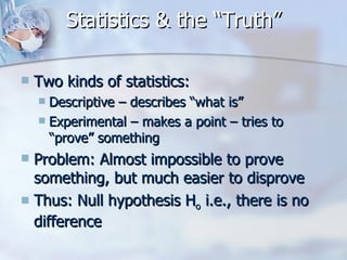
![Statistics and the “Truth” Can we ever know the truth? Statistics is a way of telling us the likelihood that we have arrived at the truth of a matter [or not!].](https://image.slidesharecdn.com/introductorystatisticsforavmed-110501110208-phpapp02/85/Introductory-Statistics-4-320.jpg)
![Types of Statistics Descriptive: describe / communicate what you see without any attempts at generalizing beyond the sample at hand Inferential: determine the likelihood that observed results: Can be generalized to larger populations Occurred by chance rather than as a result of known, specified interventions [ H o ]](https://image.slidesharecdn.com/introductorystatisticsforavmed-110501110208-phpapp02/85/Introductory-Statistics-7-320.jpg)
![The Null Hypothesis A hypothesis which is tested for possible rejection under the assumption that it is true (usually that observations are the result of chance). Experimental stats works to disprove the null hypothesis, to show that the null hypothesis is wrong, that a difference exists. [e.g., glucose levels and diabetics] In other words, that you have found or discovered something new. The null hypothesis usually represents the opposite of what the researcher may believe to be true.](https://image.slidesharecdn.com/introductorystatisticsforavmed-110501110208-phpapp02/85/Introductory-Statistics-8-320.jpg)
![Variability of Measurements Unbiasedness: tendency to arrive at the true or correct value Precision: degree of spread of series of observations [repeatability] [also referred to as reliability] Can also refer to # of decimal points – can be misleading Accuracy: encompasses both unbiasedness and precision. Accurate measurements are both unbiased and precise. Inaccurate measurements may be either biased or imprecise or both.](https://image.slidesharecdn.com/introductorystatisticsforavmed-110501110208-phpapp02/85/Introductory-Statistics-14-320.jpg)
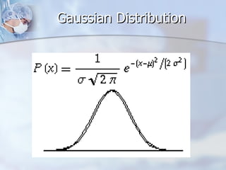
![Standard Deviation SD is a measure of scatter or dispersion of data around the mean ~68% of values fall within 1 SD of the mean [+/- one Z] ~95% of values fall within 2 SD of the mean, with ~2.5% in each tail.](https://image.slidesharecdn.com/introductorystatisticsforavmed-110501110208-phpapp02/85/Introductory-Statistics-16-320.jpg)
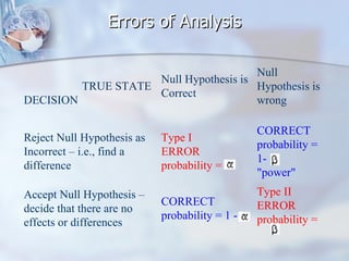
![Errors of Analysis/Detection Type 1 [alpha] error – finding a significant difference when none really exists - usually due to random error Type 2 [beta] error – not finding a difference when there is in fact a difference – more likely to occur with smaller sample sizes. Chosen significance levels will impact both of these](https://image.slidesharecdn.com/introductorystatisticsforavmed-110501110208-phpapp02/85/Introductory-Statistics-20-320.jpg)


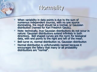
This document provides an overview of introductory statistics concepts, including: - Descriptive statistics which describe data without generalizing, versus inferential statistics which determine if results can be generalized. - The importance of the normal distribution and how it applies to statistical analyses. - Key terms like means, standard deviation, confidence intervals, types of errors, and significance testing. - Examples of common statistical tests like the t-test and how to interpret their results.