The document discusses the fundamentals and applications of policy gradient reinforcement learning, focused on maximizing future rewards through a well-defined reward function. It details various algorithms and emphasizes the importance of techniques such as variance reduction in policy gradient methods. Additionally, it touches on the MDP (Markov Decision Process) structure used in reinforcement learning, including state and action spaces, reward functions, and value functions.

1. ⽅策勾配型強化学習の
基礎と応⽤
岩城諒
2017/12/13
@KP mtg

2. • ⽬的: 未来の報酬を最⼤化する⽅策の獲得
– 設計者は”何を学習してほしいか”を報酬関数として与える
– ”どうやって達成するか”はエージェントが試⾏錯誤で獲得
– 飴/鞭を⼿掛かりに意思決定則を最適化
2
強化学習
エージェント
状態
⾏動
報酬関数
報酬
状態遷移則
⽅策
環境

3. 3
強化学習でできること
ngaging for human players. We used the same network
yperparameter values (see Extended Data Table 1) and
urethroughout—takinghigh-dimensionaldata(210|160
t 60 Hz) as input—to demonstrate that our approach
successful policies over a variety of games based solely
utswithonlyveryminimalpriorknowledge(thatis,merely
were visual images, and the number of actions available
but not their correspondences; see Methods). Notably,
as able to train large neural networks using a reinforce-
ignalandstochasticgradientdescentinastablemanner—
he temporal evolution of two indices of learning (the
e score-per-episode and average predicted Q-values; see
plementary Discussion for details).
We compared DQN with the best performing methods from the
reinforcement learning literature on the 49 games where results were
available12,15
. In addition to the learned agents, we alsoreport scores for
aprofessionalhumangamestesterplayingundercontrolledconditions
and a policy that selects actions uniformly at random (Extended Data
Table 2 and Fig. 3, denoted by 100% (human) and 0% (random) on y
axis; see Methods). Our DQN method outperforms the best existing
reinforcement learning methods on 43 of the games without incorpo-
rating any of the additional prior knowledge about Atari 2600 games
used by other approaches (for example, refs 12, 15). Furthermore, our
DQN agent performed at a level that was comparable to that of a pro-
fessionalhumangamestesteracrossthesetof49games,achievingmore
than75%ofthe humanscore onmorethanhalfofthegames(29 games;
Convolution Convolution Fully connected Fully connected
No input
matic illustration of the convolutional neural network. The
hitecture are explained in the Methods. The input to the neural
s of an 843 843 4 image produced by the preprocessing
by three convolutional layers (note: snaking blue line
symbolizes sliding of each filter across input image) and two fully connected
layers with a single output for each valid action. Each hidden layer is followed
by a rectifier nonlinearity (that is, max 0,xð Þ).
a b
c d
0
200
400
600
800
1,000
1,200
1,400
1,600
1,800
2,000
2,200
0 20 40 60 80 100 120 140 160 180 200
Averagescoreperepisode
Training epochs
8
9
10
11
lue(Q)
0
1,000
2,000
3,000
4,000
5,000
6,000
0 20 40 60 80 100 120 140 160 180 200
Averagescoreperepisode
Training epochs
7
8
9
10
alue(Q)
LETTER
ゲーム [Mnih+ 15]
IEEE ROBOTICS & AUTOMATION MAGAZINE MARCH 2016104
sampled from real systems. On the other hand, if the environ-
ment is extremely stochastic, a limited amount of previously
acquired data might not be able to capture the real environ-
ment’s property and could lead to inappropriate policy up-
dates. However, rigid dynamics models, such as a humanoid
robot model, do not usually include large stochasticity. There-
fore, our approach is suitable for a real robot learning for high-
dimensional systems like humanoid robots.
formance. We proposed recursively using the off-policy
PGPE method to improve the policies and applied our ap-
proach to cart-pole swing-up and basketball-shooting
tasks. In the former, we introduced a real-virtual hybrid
task environment composed of a motion controller and vir-
tually simulated cart-pole dynamics. By using the hybrid
environment, we can potentially design a wide variety of
different task environments. Note that complicated arm
movements of the humanoid robot need to be learned for
the cart-pole swing-up. Furthermore, by using our pro-
posed method, the challenging basketball-shooting task
was successfully accomplished.
Future work will develop a method based on a transfer
learning [28] approach to efficiently reuse the previous expe-
riences acquired in different target tasks.
Acknowledgment
This work was supported by MEXT KAKENHI Grant
23120004, MIC-SCOPE, ``Development of BMI Technolo-
gies for Clinical Application’’ carried out under SRPBS by
AMED, and NEDO. Part of this study was supported by JSPS
KAKENHI Grant 26730141. This work was also supported by
NSFC 61502339.
References
[1] A. G. Kupcsik, M. P. Deisenroth, J. Peters, and G. Neumann, “Data-effi-
cient contextual policy search for robot movement skills,” in Proc. National
Conf. Artificial Intelligence, 2013.
[2] C. E. Rasmussen and C. K. I. Williams Gaussian Processes for Machine
Learning. Cambridge, MA: MIT Press, 2006.
[3] C. G. Atkeson and S. Schaal, “Robot learning from demonstration,” in Proc.
14th Int. Conf. Machine Learning, 1997, pp. 12–20.
[4] C. G. Atkeson and J. Morimoto, “Nonparametric representation of poli-
cies and value functions: A trajectory-based approach,” in Proc. Neural Infor-
mation Processing Systems, 2002, pp. 1643–1650.Figure 13. The humanoid robot CB-i [7]. (Photo courtesy of ATR.)
ロボット制御 [Sugimoto+ 16]
IBM Research / Center for Business Optimization
Modeling and Optimization
Engine
Actions
Other
System 1
System 2
System 3
Event Listener
Event
Notification
Event
Notification
Event
Notification
< inserts >
TP Profile
Taxpayer State
( Current )
Modeler
Optimizer
< input to >
State Generator
< input to >
Case Inventory
< reads >
< input to >
Allocation Rules
Resource
Constraints
< input to >
< inserts , updates >
Business Rules
< input to >
< generates >
Segment Selector Action
1
Cnt Action
2
Cnt Action
n
Cnt
1 C
1
^ C
2
V C
3
200 50 0
2 C
4
V C
1
^ C
7
0 50 250
TP ID Feat
1
Feat
2
Feat
n
123456789 00 5 A 1500
122334456 01 0 G 1600
122118811 03 9 G 1700
Rule Processor
< input to >
< input to >
Recommended
Actions
< inserts , updates >
TP ID Rec. Date Rec. Action Start Date
123456789 00 6/21/2006 A1 6/21/2006
122334456 01 6/20/2006 A2 6/20/2006
122118811 03 5/31/2006 A2
Action Handler
< input to >
New
Case
Case Extract
Scheduler
< starts > < updates >
State
Time Expired
Event
Notification
< input to >
Taxpayer State
History
State
TP ID State Date Feat
1
Feat
2
Feat
n
123456789 00 6/1/2006 5 A 1500
122334456 01 5/31/2006 0 G 1600
122118811 03 4/16/2006 4 R 922
122118811 03 4/20/2006 9 G 1700
< inserts >
Feature Definitions
(XML)
(XSLT)
(XML)
(XML)
(XSLT)
Figure 2: Overall collections system architecture.
債権回収の最適化 [Abe+ 10]
囲碁 [Silver+ 16]

4. 4
Example :: 1
• 環境：迷路
• エージェント：
• 状態：位置
• ⾏動：↑↓←→
• 報酬：
価値関数 ⽅策
0 1 2
1 2 3 4 3 2
2 3 4 5 4 3
6 5 4
10 9 8 7 6 5
G 10 9
↓ ↓ ↓
→ ↓ ↓ ↓ ↓ ←
→ → → ↓ ↓ ←
↓ ← ←
↓ ↓ ← ← ← ←
G ← ←

5. 5
Example :: 2 :: Atari 2600
• 状態：ゲームのプレイ画⾯
• ⾏動：コントローラの操作
• 報酬：スコア
Convolution Convolution Fully connected Fully connected
No input
Figure 1 | Schematic illustration of the convolutional neural network. The symbolizes sliding of each filter across input image) and two fu
RESEARCH LETTER
[Mnih+ 15]
LETTER RESEARCH

6. 6
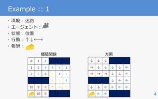
Example :: 3 :: Basketball Shooting
• 状態：ロボットの関節⾓度（使ってない）
• ⾏動：関節⾓度の⽬標値
• 報酬：ゴールからの距離
dimensional dynamics models with a limited amount of data
sampled from real systems. On the other hand, if the environ-
ment is extremely stochastic, a limited amount of previously
acquired data might not be able to capture the real environ-
ment’s property and could lead to inappropriate policy up-
dates. However, rigid dynamics models, such as a humanoid
robot model, do not usually include large stochasticity. There-
fore, our approach is suitable for a real robot learning for high-
dimensional systems like humanoid robots.
es of a humanoid robot to eff
formance. We proposed recu
PGPE method to improve the
proach to cart-pole swing-u
tasks. In the former, we intr
task environment composed o
tually simulated cart-pole dy
environment, we can potenti
different task environments.
movements of the humanoid
the cart-pole swing-up. Furt
posed method, the challengi
was successfully accomplished
Future work will develop a
learning [28] approach to effici
riences acquired in different tar
Acknowledgment
This work was supported b
23120004, MIC-SCOPE, ``De
gies for Clinical Application’’
AMED, and NEDO. Part of thi
KAKENHI Grant 26730141. Th
NSFC 61502339.
References
[1] A. G. Kupcsik, M. P. Deisenroth, J.
cient contextual policy search for robo
Conf. Artificial Intelligence, 2013.
[2] C. E. Rasmussen and C. K. I. Will
Learning. Cambridge, MA: MIT Press, 2
[3] C. G. Atkeson and S. Schaal, “Robot
14th Int. Conf. Machine Learning, 1997, pp
[4] C. G. Atkeson and J. Morimoto, “N
cies and value functions: A trajectory-b
mation Processing Systems, 2002, pp. 164Figure 13. The humanoid robot CB-i [7]. (Photo courtesy of ATR.)
our proposed approach,
we compared the following methods:
● REINFORCE: The REINFORCE algorithm [25]
● PGPE: Standard PGPE [6]
● IW-PGPE: Standard IW-PGPE [34]
● Proposed: Proposed recursive IW-PGPE.
For each method, we updated the parameters every ten trials
and used the same learning rate.
2 m
(a)
0.9 m
0.5 m
0.5 m
0.1 m
y
z
x
Robot
i5, i6, i7
p(xp, yp, zp = 0.5) i1, i2, i3
i4
[Sugimoto+ 16]

7. 7
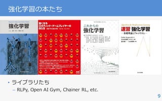
Example :: 4 :: Go
• 状態：盤⾯
• ⾏動：次に打つ⼿
• 報酬：勝敗
[Silver+ 16]
ARTICLE RESEARC
and architecture. a, A fast the current player wins) in positions from the self-play data set.
Regression
SelfPlay
radient
b
Self-play positions
NeuralnetworkData
p (a⎪s) (s′)p
RL policy network Value network Policy network Value network
s s′
phaGo than a value function ( )≈ ( )θ σv s v sp derived from the
etwork.
ng policy and value networks requires several orders of
more computation than traditional search heuristics. To
combine MCTS with deep neural networks, AlphaGo uses
onous multi-threaded search that executes simulations on
computes policy and value networks in parallel on GPUs.
ersion of AlphaGo used 40 search threads, 48 CPUs, and
e also implemented a distributed version of AlphaGo that
exploited multiple machines, 40 search thre
176 GPUs. The Methods section provides full d
and distributed MCTS.
Evaluating the playing strength of Alp
To evaluate AlphaGo, we ran an internal tourn
of AlphaGo and several other Go programs, i
commercial programs Crazy Stone13
and Zen,
source programs Pachi14
and Fuego15
. All of th
Principal variation
Value networka
fPolicy network Percentage of simulations
b c Tree evaluation from rolloutsTree evaluation from value net
d e g

8. 8
内容
• ⽅策勾配型強化学習のざっくりとした説明
– ⽅策勾配の理論的な側⾯に着⽬
– 実際のアルゴリズムなどについてはほぼ触れない
– Variance Reduction も⾮常に重要だがパス
• 基礎：これをおさえればほぼ勝ち
– REINFORCE [Williams 92]
– ⽅策勾配定理 [Sutton+ 99]
• 応⽤：⽅策勾配定理からの様々な派⽣

9. 9
強化学習の本たち
• ライブラリたち
– RLPy, Open AI Gym, Chainer RL, etc.

10. 10
Notation :: Markov Decision Process
• マルコフ決定過程 / MDP
• 状態・⾏動空間
• 状態遷移則
• 報酬関数
• 初期状態分布
• 割引率
• ⽅策
• 状態の分布
Agent
Environment
state actionreward
S, A
P : S ⇥ A ⇥ S ! R
R : S ⇥ A ! [ Rmax, Rmax]
⇢0 : S ! R
2 [0, 1)
(S, A, P, R, ⇢0, )
⇡ : S ⇥ A ! R or ⇡ : S ! A
⇢⇡
(s) =
1X
t=0
t
Pr (st = s|⇢0, ⇡)

11. 11
価値関数たち
• 状態価値・⾏動価値・アドバンテージ
– 未来の報酬の予測値
– ある状態・⾏動がどれだけ良い/悪いかを表す
– 状態・⾏動空間での ”地図”
状態価値関数
0 1 2
1 2 3 4 3 2
2 3 4 5 4 3
6 5 4
10 9 8 7 6 5
G 10 9
V ⇡
(s) = E
" 1X
t=0
t
R(st, at) |s0 = s
#
Q⇡
(s, a) = R(s, a) +
X
s02S
P(s0
|s, a)V ⇡
(s0
)
V ⇡
(s) =
X
a2A
⇡(a|s)Q⇡
(s, a)

12. 12
価値関数たち
• アドバンテージ
=
s, a
Q⇡
s
V ⇡
A⇡
s, a
A⇡
(s, a) = Q⇡
(s, a) V ⇡
(s)
X
a2A
⇡(a|s)A⇡
(s, a) =
X
a2A
⇡(a|s) (Q⇡
(s, a) V ⇡
(s))
= V ⇡
(s) V ⇡
(s) = 0

13. 13
MDPを解く
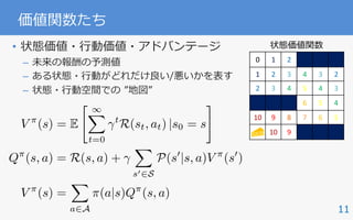
• 強化学習の⽬的: 価値を最⼤化する最適⽅策の獲得
• MDPには最適価値関数 が⼀意に存在し，
少なくとも⼀つの最適な決定論的⽅策が存在する．
– greedy⽅策：常に価値が最⼤になる⾏動を選ぶ
V ⇤
(s), Q⇤
(s, a)
⇡⇤
2 arg max
⇡
⌘(⇡),
where ⌘(⇡) =
X
s2S
⇢0(s)V ⇡
(s) =
X
s2S,a2A
⇢⇡
(s)⇡(a|s)R(s, a)
= E⇡ [R(s, a)]
⇡⇤
(s) = arg maxa2AQ⇤
(s, a)

14. 14
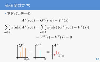
Bellman ⽅程式
P(s0
|s, a)
P(s00
|s0
, a0
)
⇡(a|s)
⇡(a0
|s0
)
s
s0
a0
a
s00
V ⇡
(s) = E
" 1X
t=0
t
R(st, at) |s0 = s
#
= E [R(s, a) |s0 = s] + E
" 1X
t=0
t
R(st+1, at+1) |s0 = s
#
=
X
a2A
⇡(a|s)R(s, a) +
X
a2A
⇡(a|s)
X
s02S
P(s0
|s, a)E
" 1X
t=0
t
R(st+1, at+1) |s1 = s0
#
=
X
a2A
⇡(a|s)R(s, a) +
X
a2A
⇡(a|s)
X
s02S
P(s0
|s, a)V ⇡
(s0
)
=
X
a2A
⇡(a|s) R(s, a) +
X
s02S
P(s0
|s, a)V ⇡
(s0
)
!

15. 15
Bellman （最適）⽅程式たち
• Bellman ⽅程式
• Bellman 最適⽅程式
V ⇡
(s) =
X
a2A
⇡(a|s) R(s, a) +
X
s02S
P(s0
|s, a)V ⇡
(s0
)
!
Q⇡
(s, a) = R(s, a) +
X
s02S
P(s0
|s, a)
X
a02A
⇡(a0
|s0
)Q⇡
(s0
, a0
)
V ⇤
(s) = max
a2A
R(s, a) +
X
s02S
P(s0
|s, a)V ⇤
(s0
)
!
Q⇤
(s, a) = R(s, a) +
X
s02S
P(s0
|s, a) max
a02A
Q⇤
(s0
, a0
)

16. 16
価値反復 / Value Iteration
• MDPの解法の⼀つ
– モデルベース：状態遷移確率と報酬関数が既知
• 価値反復 (c.f. ⽅策反復 / Policy Iteration)
1. 価値関数の初期値 を与える．
2. ベルマン最適⽅程式を適⽤:
3. ひたすら繰り返す．
• 状態価値についても同様
• 最適価値関数へ指数関数的に収束
Qk+1(s, a) = R(s, a) +
X
s02S
P(s0
|s, a) max
a02A
Qk(s0
, a0
)
Q0
Q
Q
Q
Q⇤
Q⇤
Q⇤
Q = Q⇤
Q
Q
Q
Q

17. 17
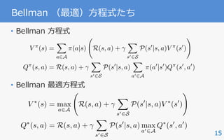
近似価値反復 / Approximate Value Iteration
• 価値反復では毎更新ですべての状態・⾏動の組を評価
– 状態・⾏動空間が⼤きくなると計算量が指数関数的に爆発
• そもそも状態遷移確率と報酬関数は⼀般に未知
• 近似価値反復
– サンプル (s,a,sʼ,r) から近似的に価値反復
– Q学習 [Watkins 89] + greedy ⽅策
Q(s, a) (1 ↵)Q(s, a) + ↵
✓
R(s, a) + max
a02A
Q(s0
, a0
)
◆
⇡(s) = arg maxa2AQ(s, a)

18. 18
⽅策探索
• 強化学習の⽬的:
価値を最⼤化する最適⽅策の獲得
• ⽅策探索 / (direct) policy search
– ⽅策を陽に表現して直接最適化
– 連続な⾏動を扱いやすい
– ロボティクスへの応⽤が盛ん
IEEE ROBOTICS & AUTOMATION MAGAZINE MARCH 2016104
mensional systems like
humanoid robots, this
problem becomes more
serious due to the difficul-
ty of approximating high-
dimensional dynamics models with a limited amount of data
sampled from real systems. On the other hand, if the environ-
ment is extremely stochastic, a limited amount of previously
acquired data might not be able to capture the real environ-
ment’s property and could lead to inappropriate policy up-
dates. However, rigid dynamics models, such as a humanoid
robot model, do not usually include large stochasticity. There-
fore, our approach is suitable for a real robot learning for high-
dimensional systems like humanoid robots.
might be inter
work as a futur
Conclusions
In this article,
es of a human
formance. We
PGPE method
proach to car
tasks. In the f
task environm
tually simulate
environment,
different task
movements of
the cart-pole
posed method
was successful
Future wor
learning [28] a
riences acquire
Acknowledg
This work wa
23120004, MIC
gies for Clinic
AMED, and N
KAKENHI Gra
NSFC 6150233
References
[1] A. G. Kupcsik,
cient contextual po
Conf. Artificial Inte
[2] C. E. Rasmusse
Learning. Cambrid
[3] C. G. Atkeson a
14th Int. Conf. Mach
[4] C. G. Atkeson
cies and value func
mation Processing S
environments.
Figure 13. The humanoid robot CB-i [7]. (Photo courtesy of ATR.)
[Sugimoto+ 16]

19. 19
⽅策勾配法 / Policy Gradient Method
• 確率的⽅策を関数近似：
– すべての⾏動の確率（密度）が正 & θについて微分可能
– tile coding（離散化），RBFネットワーク，ニューラルネットワーク
• ⽬的関数を⽅策パラメータに
ついて微分し勾配法で学習
• これ以後の内容は全て
⽅策勾配 の推定⽅法
✓0
= ✓ + ↵r✓⌘(⇡✓)
r✓⌘(⇡✓)
⌘(⇡✓0 )
⌘(⇡✓⇤ )
⌘(⇡✓)
✓⇤
✓
r✓⌘(⇡✓)
✓0
⇡ , ⇡✓

20. 20
REINFORCE
• [Williams 92]
• REward Increment
= Nonnegative Factor x Offset Reinforcement
x Characteristic Eligibility
• 勾配を不偏推定
• b: ベースライン
• ⽅策勾配法の興り
• Alpha Goの⾃⼰対戦で⽤いられた
✓0
= ✓ + ↵ (r b) r✓ ln ⇡✓(a|s)
r✓⌘(⇡✓)

21. 21
REINFORCE :: 導出 :: 1
• を仮定（成り⽴つはずがない）
r✓⌘(⇡) = r✓E⇡ [R(s, a)]
= r✓
X
s2S,a2A
⇢⇡
(s)⇡✓(a|s)R(s, a)
'
X
s2S,a2A
⇢⇡
(s)r✓⇡✓(a|s)R(s, a)
=
X
s2S,a2A
⇢⇡
(s)⇡✓(a|s)
r✓⇡✓(a|s)
⇡✓(a|s)
R(s, a)
= E⇡ [r✓ ln ⇡✓(a|s)R(s, a)]
r✓⇢⇡
(s) = 0
(ln x)0
=
x0
x

22. 22
REINFORCE :: 導出 :: 2
• ⾏動に⾮依存なベースライン b は以下を満たす:
• よって
r✓
X
s2S,a2A
⇢⇡
(s)⇡✓(a|s)b(s) =
X
s2S
⇢⇡
(s)b(s)r✓
X
a2A
⇡✓(a|s)
=
X
s2S
⇢⇡
(s)b(s)r✓1 = 0
r✓⌘(⇡) = E⇡ [r✓ ln ⇡✓(a|s)R(s, a)]
= E⇡ [r✓ ln ⇡✓(a|s) (R(s, a) b(s))]

23. 23
⽅策勾配定理 / Policy Gradient Theorem
• [Sutton+ 99]
• この定理を利⽤するのがいわゆる”⽅策勾配法”．
• 即時報酬ではなく，価値（未来の報酬の予測値）を
使って⽅策勾配を推定できる．
• [Baxter & Bartlett 01]も等価
r✓⌘(⇡) = E⇡ [r✓ ln ⇡✓(a|s)Q⇡
(s, a)]

24. r✓V ⇡
(s) = r✓
X
a2A
⇡✓(a|s)Q⇡
(s, a)
=
X
a2A
[r✓⇡✓(a|s)Q⇡
(s, a) + ⇡✓(a|s)r✓Q⇡
(s, a)]
=
X
a2A
"
r✓⇡✓(a|s)Q⇡
(s, a) + ⇡✓(a|s)r✓ R(s, a) +
X
s02S
P(s0
|s, a)V ⇡
(s0
)
!#
=
X
a2A
"
r✓⇡✓(a|s)Q⇡
(s, a) + ⇡✓(a|s)
X
s02S
P(s0
|s, a)r✓
X
a02A
⇡✓(a0
|s0
)Q⇡
(s0
, a0
)
#
=
X
s02S
1X
t=0
t
Pr(st = s0
|s0 = s, ⇡)
X
a2A
r✓⇡✓(a|s0
)Q⇡
(s0
, a)
24
⽅策勾配定理 :: 導出 :: 1

25. 25
⽅策勾配定理 :: 導出 :: 2
r✓⌘(⇡) =
X
s2S
1X
t=0
t
Pr(st = s|⇢0, ⇡)
X
a2A
r✓⇡✓(a|s)Q⇡
(s, a)
=
X
s2S
⇢⇡
(s)
X
a2A
r✓⇡✓(a|s)Q⇡
(s, a)
= E⇡ [r✓ ln ⇡✓(a|s)Q⇡
(s, a)]

26. 26
⽅策勾配定理
• ⽅策勾配は様々な形式で不偏推定できる:
r✓⌘(⇡) = E⇡ [r✓ ln ⇡✓(a|s)Q⇡
(s, a)]
= E⇡ [r✓ ln ⇡✓(a|s) (Q⇡
(s, a) V ⇡
(s))]
= E⇡ [r✓ ln ⇡✓(a|s)A⇡
(s, a)]
= E⇡ [r✓ ln ⇡✓(a|s) ⇡
]
=
s, a
Q⇡
s
V ⇡
A⇡
s, a
A⇡
(s, a) = Q⇡
(s, a) V ⇡
(s)
= R(s, a) +
X
s02S
P(s0
|s, a)V ⇡
(s0
) V ⇡
(s)
= Es0⇠P [r + V ⇡
(s0
) V ⇡
(s)] = Es0⇠P [ ⇡
]<latexit sha1_base64="JdGziPix+c0H39/n+OmPaMIjE1w=">AAAGaXiclVRLb9NAEB4HGkp4tCmXilwsoqStKNGm4i0hFRASxzxIWilOo7WzSaz4JdsJFJMLR/4AB04gIYE4wV/gwh/g0J+A4FYkLhwYr02TNM9uZO/M7HzffDOOVrY01XEJORAip04vRM8sno2dO3/h4tJyfKXsmB1bYSXF1Ex7V6YO01SDlVzV1diuZTOqyxrbkdsP/fOdLrMd1TSeuPsWq+q0aagNVaEuhmpxIXF/T7LUdWeTbsTS98T8kSdeE8uBsxGTJP9M0qnbUqjmFXpBxlVRalJdp6LkdPSa56xJqnGUVOz1+ogcItZecFB5z0NW359UQpa9Rz1O56j6AAXyaazhVux+4RA+RCXZarPlVmMppEylY3OSilKdaS4NxIUUteUkyRC+xFEjGxpJCFfOjEcSIEEdTFCgAzowMMBFWwMKDv4qkAUCFsaq4GHMRkvl5wx6EENsB7MYZlCMtvHdRK8SRg30fU6HoxWsouFjI1KEFPlOPpJD8o18Ij/I34lcHufwtezjLgdYZtWWXq0W/8xE6bi70Oqjpmp2oQG3uVYVtVs84nehBPju89eHxbuFlJcm78hP1P+WHJCv2IHR/a28z7PCmyl6ZNQSTKyOfoNXYAMz8fibYrTJZ+vPS8ee29wmsIlPBm7gnsU98AM+n+cpZ9J5vwZW8DA+zOd/ySqP+z094195cu0kZvdm6K3z/0MbO9Ow51HN2VDzTb7P1jvKN13zuPon0W1jvD5m0hnYGpry/Mr/M86nu19/UPWkGvNxn4xz3kmPmTDeNNnj98qoUdrK3MmQ/PXk9oPwylmEBFyBdSS5BdvwGHJQAkV4KXwQPgtfFn5FV6Kr0ctBakQIMZdgaEWT/wC35HkI</latexit><latexit sha1_base64="JdGziPix+c0H39/n+OmPaMIjE1w=">AAAGaXiclVRLb9NAEB4HGkp4tCmXilwsoqStKNGm4i0hFRASxzxIWilOo7WzSaz4JdsJFJMLR/4AB04gIYE4wV/gwh/g0J+A4FYkLhwYr02TNM9uZO/M7HzffDOOVrY01XEJORAip04vRM8sno2dO3/h4tJyfKXsmB1bYSXF1Ex7V6YO01SDlVzV1diuZTOqyxrbkdsP/fOdLrMd1TSeuPsWq+q0aagNVaEuhmpxIXF/T7LUdWeTbsTS98T8kSdeE8uBsxGTJP9M0qnbUqjmFXpBxlVRalJdp6LkdPSa56xJqnGUVOz1+ogcItZecFB5z0NW359UQpa9Rz1O56j6AAXyaazhVux+4RA+RCXZarPlVmMppEylY3OSilKdaS4NxIUUteUkyRC+xFEjGxpJCFfOjEcSIEEdTFCgAzowMMBFWwMKDv4qkAUCFsaq4GHMRkvl5wx6EENsB7MYZlCMtvHdRK8SRg30fU6HoxWsouFjI1KEFPlOPpJD8o18Ij/I34lcHufwtezjLgdYZtWWXq0W/8xE6bi70Oqjpmp2oQG3uVYVtVs84nehBPju89eHxbuFlJcm78hP1P+WHJCv2IHR/a28z7PCmyl6ZNQSTKyOfoNXYAMz8fibYrTJZ+vPS8ee29wmsIlPBm7gnsU98AM+n+cpZ9J5vwZW8DA+zOd/ySqP+z094195cu0kZvdm6K3z/0MbO9Ow51HN2VDzTb7P1jvKN13zuPon0W1jvD5m0hnYGpry/Mr/M86nu19/UPWkGvNxn4xz3kmPmTDeNNnj98qoUdrK3MmQ/PXk9oPwylmEBFyBdSS5BdvwGHJQAkV4KXwQPgtfFn5FV6Kr0ctBakQIMZdgaEWT/wC35HkI</latexit><latexit sha1_base64="JdGziPix+c0H39/n+OmPaMIjE1w=">AAAGaXiclVRLb9NAEB4HGkp4tCmXilwsoqStKNGm4i0hFRASxzxIWilOo7WzSaz4JdsJFJMLR/4AB04gIYE4wV/gwh/g0J+A4FYkLhwYr02TNM9uZO/M7HzffDOOVrY01XEJORAip04vRM8sno2dO3/h4tJyfKXsmB1bYSXF1Ex7V6YO01SDlVzV1diuZTOqyxrbkdsP/fOdLrMd1TSeuPsWq+q0aagNVaEuhmpxIXF/T7LUdWeTbsTS98T8kSdeE8uBsxGTJP9M0qnbUqjmFXpBxlVRalJdp6LkdPSa56xJqnGUVOz1+ogcItZecFB5z0NW359UQpa9Rz1O56j6AAXyaazhVux+4RA+RCXZarPlVmMppEylY3OSilKdaS4NxIUUteUkyRC+xFEjGxpJCFfOjEcSIEEdTFCgAzowMMBFWwMKDv4qkAUCFsaq4GHMRkvl5wx6EENsB7MYZlCMtvHdRK8SRg30fU6HoxWsouFjI1KEFPlOPpJD8o18Ij/I34lcHufwtezjLgdYZtWWXq0W/8xE6bi70Oqjpmp2oQG3uVYVtVs84nehBPju89eHxbuFlJcm78hP1P+WHJCv2IHR/a28z7PCmyl6ZNQSTKyOfoNXYAMz8fibYrTJZ+vPS8ee29wmsIlPBm7gnsU98AM+n+cpZ9J5vwZW8DA+zOd/ySqP+z094195cu0kZvdm6K3z/0MbO9Ow51HN2VDzTb7P1jvKN13zuPon0W1jvD5m0hnYGpry/Mr/M86nu19/UPWkGvNxn4xz3kmPmTDeNNnj98qoUdrK3MmQ/PXk9oPwylmEBFyBdSS5BdvwGHJQAkV4KXwQPgtfFn5FV6Kr0ctBakQIMZdgaEWT/wC35HkI</latexit>

27. 27
Actor-Critic
• Actor (= ⽅策)
– 環境に対して⾏動を出⼒(act)する
• Critic (= 価値関数)
– actor のとった⾏動を
Temporal Difference (TD) 誤差
などで評価(criticize)する
• 特定の学習則というよりは，
学習器の構造を指す．
• 理論解析
– [Kimura & Kobayashi 98]
– [Konda & Tsitsiklis 00] エージェント
TD 誤
差
環境
Actor
Critic
報酬
t
TD誤差
V (s), Q(s, a)
⇡✓(a|s)
状態 ⾏動

28. 28
A3C
• [Mnih+ 16]
• Asynchronous Advantage Actor Critic
– advantage actor critic:
– asynchronous:
‣ actor-criticのペアを複数⽤意
‣ 各actor-criticが独⽴に環境と相互作⽤して勾配を計算
– （ は陽に推定せず，状態価値関数で近似）
‣ ときどき
• 膨⼤な計算資源による暴⼒
i 2 {1, N}
✓0
= ✓ + ↵ d✓
✓i = ✓0
r✓⌘(⇡) = E⇡ [r✓ ln ⇡✓(a|s)A⇡
(s, a)]
A(st, at)
d✓ d✓ + r✓i
ln ⇡✓i
(at|st)Ai
(st, at)

29. 29
Extension: (N)PGPE
• (Natural) Policy Gradient with Parameter based Exploration
[Sehnke+ 10; Miyamae+ 10]
[Zhao+ 12]
µ✓
✓
⇡(a|s; ✓)
a
s
s
p(✓|⇢)
✓
✓
PGPE
PG Var[r✓
ˆJ(✓)]
Var[r⇢
ˆJ(⇢)]


30. 30
Off-Policy Learning (<---> On-Policy)
• 学習 期待値演算
• Off-policy: 推定⽅策 挙動⽅策
• Off-policyで学習できればデータの再利⽤が可能 !!!
[Sugimoto+ 16]
E
⇡
[·] 6= E[·]
time at
with 0.00
The t
was 2 m
0.11 m)
reward i
ballandt
where th
ball’s po
( 100a =
cost was
where c
pendent
For o
cursive u
tively. T
.0 99c =
The l
ing conv
stage, th
went in.
The m
ries of th
are show
nated joi
ketball-s
the mov
tainty of
ing is sho
Discuss
In our P
istic and
Thus, th
can be
Convolution Convolution Fully connected Fully connected
No input
Figure 1 | Schematic illustration of the convolutional neural network. The
details of the architecture are explained in the Methods. The input to the neural
symbolizes sliding of each filter across input image) and two fully connected
layers with a single output for each valid action. Each hidden layer is followed
RESEARCH LETTER
[Mnih+ 15]
LETTER RESEARCH
6=
;

31. 31
Off-Policy ⽅策勾配法
• [Degris+ 12]
• 重点サンプリングを⽤いることで，
off-policyのサンプルから⽅策勾配を推定
O↵-Policy Actor-Critic
ˆZ = {u 2 U | dg(u) = 0} and the value function
weights, vt, converge to the corresponding TD-solution
with probability one.
Proof Sketch: We follow a similar outline to the
two timescale analysis for on-policy policy gradient
actor-critic (Bhatnagar et al., 2009) and for nonlinear
GTD (Maei et al., 2009). We analyze the dynamics
for our two weights, ut and zt
T
= (wt
T
vt
T
), based on
our update rules. The proof involves satisfying seven
requirements from Borkar (2008, p. 64) to ensure con-
vergence to an asymptotically stable equilibrium.
4. Empirical Results
Behavior
Softmax-GQ
O↵-Policy Actor-Critic
= 0} and the value function
the corresponding TD-solution
ollow a similar outline to the
for on-policy policy gradient
et al., 2009) and for nonlinear
9). We analyze the dynamics
and zt
T
= (wt
T
vt
T
), based on
proof involves satisfying seven
kar (2008, p. 64) to ensure con-
tically stable equilibrium.
ults
Behavior Greedy-GQ
Softmax-GQ O↵-PAC
⌘ (⇡✓) ,
X
s2S
⇢ (s)V ⇡
(s)
r✓⌘ (⇡✓) '
X
s2S
⇢ (s)
X
a2A
r✓⇡✓(a|s)Q⇡
(s, a)
=
X
s2S
⇢ (s)
X
a2A
(a|s)
⇡✓(a|s)
(a|s)
r✓⇡✓(a|s)
⇡✓(a|s)
Q⇡
(s, a)
= E

⇡✓(a|s)
(a|s)
r✓ ln ⇡✓(a|s)Q⇡
(s, a)

32. 32
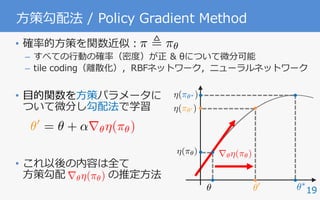
Deterministic Policy Gradient
• [Silver+ 14]
• 決定的⽅策 μ についての⽅策勾配定理
• Off-policy Deterministic Policy Gradient
• Criticとして保持している⾏動価値関数の勾配で学習
r✓⌘(µ✓) = Es⇠⇢µ
⇥
r✓µ✓(s)raQµ
(s, a)|a=µ(s)
⇤
r✓⌘ (µ✓) = Es⇠⇢
⇥
r✓µ✓(s)raQµ
(s, a)|a=µ(s)
⇤

33. 33
Deterministic Policy Gradient
• ⾏動が確率変数でないため，
– 重点サンプリングが不要・勾配推定の分散が⼩さい
– 状態のみについての期待値計算であるため学習が早い
10
2
10
3
10
4
10
−4
10
−3
10
−2
10
−1
10
0
10
1
10
Time−steps
SAC−B
COPDAC−B
10
2
10
3
10
4
10
−4
10
−3
10
−2
10
−1
10
0
10
1
10
Time−steps
10
4
stic actor-critic (SAC-B) and deterministic actor-critic (COPDAC-B) on the continuous bandit task.
0.0 10.0 20.0 30.0 40.0 50.0
Time-steps (x10000)
-6.0
-4.0
-2.0
0.0
2.0
4.0
6.0
TotalRewardPerEpisode
(x1000)
COPDAC-Q
SAC
OffPAC-TD
r✓⌘ (µ✓) = Es⇠⇢
⇥
r✓µ✓(s)raQµ
(s, a)|a=µ(s)
⇤

34. 34
⽅策を単調改善したい
• Policy oscillation
/ Policy degradation
• 関数近似の下で
⽅策の単調改善を⽬指した研究たち:
– Conservative Policy Iteration [Kakade & Langford 02]
– Safe Policy Iteration [Pirotta+ 13]
– Trust Region Policy Optimization [Schulman+ 15]
58 P. Wagner / Neural Networks 52 (2014) 43–61
(a) Performance level of the policy after each policy update.
[Bertsekas 11; Wagner 11; 14]

35. 35
Trust Region Policy Optimization
• [Schulman+ 15]
• 任意の⽅策 π と πʼ について:
• ⽅策 πʼ を実際にサンプリングすることなく評価できる
• 右辺が正であれば⽅策は単調改善
: πʼ の π に対するアドバンテージ
: πʼ と π の 分離度
⌘(⇡0
) ⌘(⇡)
X
s2S
⇢⇡
(s) ¯A⇡
⇡0 (s) c Dmax
KL (⇡0
k⇡)
¯A⇡
⇡0 (s) =
X
a2A
⇡0
(a|s)A⇡
(s, a),
Dmax
KL (⇡0
k⇡) = max
s2S
DKL(⇡0
(·|s)k⇡(·|s))

36. 36
Trust Region Policy Optimization
• Trust Region Policy Optimization [Schulman+ 15]
– 以下の制約付き最適化問題の解として⽅策を更新
• Proximal Policy Optimization [Schulman+ 17a]
– 制約付き最適化ではなく正則化として，勾配法で学習
– の値をある範囲で打ち切ることで学習を安定化
maximize
✓0
L(✓0
, ✓) = Es⇠⇢✓,a⇠⇡✓

⇡✓0 (a|s)
⇡✓(a|s)
A⇡✓
(a|s)
subject to Es⇠⇢✓ [DKL(⇡✓(·|s)k⇡✓0 (·|s))] 
⇡✓0 (a|s)/⇡✓(a|s)
LPPO
(✓0
, ✓) = Es⇠⇢✓,a⇠⇡✓

⇡✓0 (a|s)
⇡✓(a|s)
A⇡✓
(a|s) c Es⇠⇢✓ [DKL(⇡✓(·|s)k⇡✓0 (·|s))]

37. 37
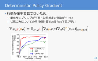
Benchmarking
• [Duan+ 16]
• Mujoco
Benchmarking Deep Reinforcement L
(a) (b) (c) (d)
F
F

38. 38
Benchmarking
ble 1. Performance of the implemented algorithms in terms of average return over all training iterations for five different random seeds (same across all algorithms). The results
the best-performing algorithm on each task, as well as all algorithms that have performances that are not statistically significantly different (Welch’s t-test with p < 0.05), are
hlighted in boldface.a
In the tasks column, the partially observable variants of the tasks are annotated as follows: LS stands for limited sensors, NO for noisy observations and
ayed actions, and SI for system identifications. The notation N/A denotes that an algorithm has failed on the task at hand, e.g., CMA-ES leading to out-of-memory errors in the
l Humanoid task.
Task Random REINFORCE TNPG RWR REPS TRPO CEM CMA-ES DDPG
Cart-Pole Balancing 77.1 ± 0.0 4693.7 ± 14.0 3986.4 ± 748.9 4861.5 ± 12.3 565.6 ± 137.6 4869.8 ± 37.6 4815.4 ± 4.8 2440.4 ± 568.3 4634.4 ± 87.8
Inverted Pendulum* 153.4 ± 0.2 13.4 ± 18.0 209.7 ± 55.5 84.7 ± 13.8 113.3 ± 4.6 247.2 ± 76.1 38.2 ± 25.7 40.1 ± 5.7 40.0 ± 244.6
Mountain Car 415.4 ± 0.0 67.1 ± 1.0 -66.5 ± 4.5 79.4 ± 1.1 275.6 ± 166.3 -61.7 ± 0.9 66.0 ± 2.4 85.0 ± 7.7 288.4 ± 170.3
Acrobot 1904.5 ± 1.0 508.1 ± 91.0 395.8 ± 121.2 352.7 ± 35.9 1001.5 ± 10.8 326.0 ± 24.4 436.8 ± 14.7 785.6 ± 13.1 -223.6 ± 5.8
Double Inverted Pendulum* 149.7 ± 0.1 4116.5 ± 65.2 4455.4 ± 37.6 3614.8 ± 368.1 446.7 ± 114.8 4412.4 ± 50.4 2566.2 ± 178.9 1576.1 ± 51.3 2863.4 ± 154.0
Swimmer* 1.7 ± 0.1 92.3 ± 0.1 96.0 ± 0.2 60.7 ± 5.5 3.8 ± 3.3 96.0 ± 0.2 68.8 ± 2.4 64.9 ± 1.4 85.8 ± 1.8
Hopper 8.4 ± 0.0 714.0 ± 29.3 1155.1 ± 57.9 553.2 ± 71.0 86.7 ± 17.6 1183.3 ± 150.0 63.1 ± 7.8 20.3 ± 14.3 267.1 ± 43.5
2D Walker 1.7 ± 0.0 506.5 ± 78.8 1382.6 ± 108.2 136.0 ± 15.9 37.0 ± 38.1 1353.8 ± 85.0 84.5 ± 19.2 77.1 ± 24.3 318.4 ± 181.6
Half-Cheetah 90.8 ± 0.3 1183.1 ± 69.2 1729.5 ± 184.6 376.1 ± 28.2 34.5 ± 38.0 1914.0 ± 120.1 330.4 ± 274.8 441.3 ± 107.6 2148.6 ± 702.7
Ant* 13.4 ± 0.7 548.3 ± 55.5 706.0 ± 127.7 37.6 ± 3.1 39.0 ± 9.8 730.2 ± 61.3 49.2 ± 5.9 17.8 ± 15.5 326.2 ± 20.8
Simple Humanoid 41.5 ± 0.2 128.1 ± 34.0 255.0 ± 24.5 93.3 ± 17.4 28.3 ± 4.7 269.7 ± 40.3 60.6 ± 12.9 28.7 ± 3.9 99.4 ± 28.1
Full Humanoid 13.2 ± 0.1 262.2 ± 10.5 288.4 ± 25.2 46.7 ± 5.6 41.7 ± 6.1 287.0 ± 23.4 36.9 ± 2.9 N/A ± N/A 119.0 ± 31.2
Cart-Pole Balancing (LS)* 77.1 ± 0.0 420.9 ± 265.5 945.1 ± 27.8 68.9 ± 1.5 898.1 ± 22.1 960.2 ± 46.0 227.0 ± 223.0 68.0 ± 1.6
Inverted Pendulum (LS) 122.1 ± 0.1 13.4 ± 3.2 0.7 ± 6.1 107.4 ± 0.2 87.2 ± 8.0 4.5 ± 4.1 81.2 ± 33.2 62.4 ± 3.4
Mountain Car (LS) 83.0 ± 0.0 81.2 ± 0.6 -65.7 ± 9.0 81.7 ± 0.1 82.6 ± 0.4 -64.2 ± 9.5 -68.9 ± 1.3 -73.2 ± 0.6
Acrobot (LS)* 393.2 ± 0.0 128.9 ± 11.6 -84.6 ± 2.9 235.9 ± 5.3 379.5 ± 1.4 -83.3 ± 9.9 149.5 ± 15.3 159.9 ± 7.5
Cart-Pole Balancing (NO)* 101.4 ± 0.1 616.0 ± 210.8 916.3 ± 23.0 93.8 ± 1.2 99.6 ± 7.2 606.2 ± 122.2 181.4 ± 32.1 104.4 ± 16.0
Inverted Pendulum (NO) 122.2 ± 0.1 6.5 ± 1.1 11.5 ± 0.5 110.0 ± 1.4 119.3 ± 4.2 10.4 ± 2.2 55.6 ± 16.7 80.3 ± 2.8
Mountain Car (NO) 83.0 ± 0.0 74.7 ± 7.8 -64.5 ± 8.6 81.7 ± 0.1 82.9 ± 0.1 -60.2 ± 2.0 67.4 ± 1.4 73.5 ± 0.5
Acrobot (NO)* 393.5 ± 0.0 -186.7 ± 31.3 -164.5 ± 13.4 233.1 ± 0.4 258.5 ± 14.0 -149.6 ± 8.6 213.4 ± 6.3 236.6 ± 6.2
Cart-Pole Balancing (SI)* 76.3 ± 0.1 431.7 ± 274.1 980.5 ± 7.3 69.0 ± 2.8 702.4 ± 196.4 980.3 ± 5.1 746.6 ± 93.2 71.6 ± 2.9
Inverted Pendulum (SI) 121.8 ± 0.2 5.3 ± 5.6 14.8 ± 1.7 108.7 ± 4.7 92.8 ± 23.9 14.1 ± 0.9 51.8 ± 10.6 63.1 ± 4.8
Mountain Car (SI) 82.7 ± 0.0 63.9 ± 0.2 -61.8 ± 0.4 81.4 ± 0.1 80.7 ± 2.3 -61.6 ± 0.4 63.9 ± 1.0 66.9 ± 0.6
Acrobot (SI)* 387.8 ± 1.0 -169.1 ± 32.3 -156.6 ± 38.9 233.2 ± 2.6 216.1 ± 7.7 -170.9 ± 40.3 250.2 ± 13.7 245.0 ± 5.5
Swimmer + Gathering 0.0 ± 0.0 0.0 ± 0.0 0.0 ± 0.0 0.0 ± 0.0 0.0 ± 0.0 0.0 ± 0.0 0.0 ± 0.0 0.0 ± 0.0 0.0 ± 0.0
Ant + Gathering 5.8 ± 5.0 0.1 ± 0.1 0.4 ± 0.1 5.5 ± 0.5 6.7 ± 0.7 0.4 ± 0.0 4.7 ± 0.7 N/A ± N/A 0.3 ± 0.3
Swimmer + Maze 0.0 ± 0.0 0.0 ± 0.0 0.0 ± 0.0 0.0 ± 0.0 0.0 ± 0.0 0.0 ± 0.0 0.0 ± 0.0 0.0 ± 0.0 0.0 ± 0.0
Ant + Maze 0.0 ± 0.0 0.0 ± 0.0 0.0 ± 0.0 0.0 ± 0.0 0.0 ± 0.0 0.0 ± 0.0 0.0 ± 0.0 N/A ± N/A 0.0 ± 0.0

39. 39
Q-Prop / Interpolated Policy Gradient
• [Gu+ 17a; 17b]
• TRPO と DPG の組み合わせ
r✓⌘(⇡✓) ⇡ (1 ⌫)Es⇠⇢✓,a⇠⇡✓
[r✓ ln ⇡✓(a|s)A⇡✓
(a|s)]
+ ⌫Es⇠⇢ [r✓Qµ✓
(s, µ✓(s))]
⇡ (1 ⌫)Es⇠⇢✓,a⇠⇡✓

r✓0
⇡✓0 (a|s)
⇡✓(a|s)
|✓0=✓A⇡✓
(a|s)
+ ⌫Es⇠⇢
⇥
r✓µ✓(s)raQµ✓
(s, a)|a=µ✓(s)
⇤
⇡✓(a|s) = (a µ✓(s))

40. 40
その他の重要な学習法たち
• ACER
– [Wang+ 17]
– Off-policy Actor Critic + Retrace [Munos+ 16]
• ⽅策勾配法 と Q 学習の統⼀的理解
– [OʼDonoghue+ 17; Nachum+ 17a; Schulman+ 17b]
• Trust-PCL
– Off-Policy TRPO
– [Nachum+ 17b]
• ⾃然⽅策勾配法
– [Kakade 01]

41. 41
References :: 1
[Abe+ 10] Optimizing Debt Collections Using Constrained Reinforcement Learning, ACM SIGKDD.
[Baxter & Bartlett 01] Infinite-horizon policy-gradient estimation. JAIR.
[Bertsekas 11] Approximate policy iteration: A survey and some new methods, Journal of Control
Theory and Applications.
[Degris+ 12] Off-Policy Actor-Critic, ICML.
[Duan+ 16] Benchmarking Deep Reinforcement Learning for Continuous Control, ICML.
[Gu+ 17a] Q-prop: Sample-efficient policy gradient with an off-policy critic, ICLR.
[Gu+ 17b] Interpolated policy gradient: Merging on-policy and off-policy gradient estimation for deep
reinforcement learning, NIPS.
[Kakade 01] A Natural Policy Gradient, NIPS.
[Kakade & Langford 02] Approximately Optimal Approximate Reinforcement Learning, ICML.
[Kimura & Kobayashi 98] An analysis of actor/critic algorithms using eligibility traces, ICML.
[Konda & Tsitsiklis 00] Actor-critic algorithms, NIPS.
[Miyamae+ 10] Natural Policy Gradient Methods with Parameter-based Exploration for Control Tasks,
NIPS.
[Mnih+ 15] Human- level control through deep reinforcement learning, Nature.
[Mnih+ 16] Asynchronous Methods for Deep Reinforcement Learning, ICML.
[Munos+ 16] Safe and efficient off-policy reinforcement learning, NIPS.
[Nachum+ 17a] Bridging the Gap Between Value and Policy Based Reinforcement Learning, NIPS.

42. 42
References :: 2
[Nachum+ 17b] Trust-PCL: An Off-Policy Trust Region Method for Continuous Control, arxiv.
[OʼDonoghue+ 17] Combining Policy Gradient and Q-Learning, ICLR.
[Pirotta+ 13] Safe Policy Iteration, ICML.
[Sehnke+ 10] Parameter-exploring policy gradients, Neural Networks.
[Schulman+ 15] Trust Region Policy Optimization, ICML.
[Schulman+ 17a] Proximal Policy Optimization Algorithms, arxiv.
[Schulman+ 17b] Equivalence Between Policy Gradients and Soft Q-Learning, arxiv.
[Silver+ 14] Deterministic Policy Gradient Algorithms, ICML
[Silver+ 16] Mastering the game of Go with deep neural networks and tree search, Nature.
[Sugimoto+ 16] Trial and error: Using previous experiences as simulation models in humanoid motor
learning, IEEE Robotics & Automation Magazine.
[Sutton+ 99] Policy Gradient Methods for Reinforcement Learning with Function Approximation, NIPS.
[Wagner 11] A reinterpretation of the policy oscillation phenomenon in approximate policy iteration,
NIPS.
[Wagner 14] Policy oscillation is overshooting, Neural Networks.
[Wang+ 17] Sample efficient actor-critic with experience replay, ICLR.
[Watkins 89] Learning From Delayed Rewards, PhD Thesis.
[Williams 92] Simple Statistical Gradient-Following Algorithms for Connectionist Reinforcement
Learning, Machine Learning,