Download to read offline


![DeepFashion2: A Versatile Benchmark for Detection, Pose Estimation,
Segmentation and Re-Identification of Clothing Images
Yuying Ge1
, Ruimao Zhang1
, Lingyun Wu2
, Xiaogang Wang1
, Xiaoou Tang1
, and Ping Luo1
1
The Chinese University of Hong Kong
2
SenseTime Research
Abstract
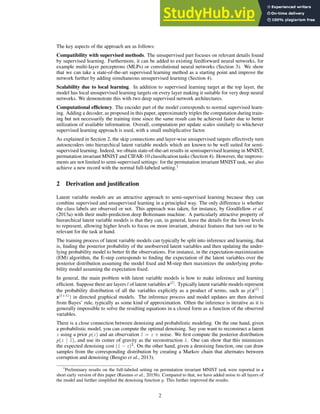
Understanding fashion images has been advanced by
benchmarks with rich annotations such as DeepFashion,
whose labels include clothing categories, landmarks, and
consumer-commercial image pairs. However, DeepFash-
ion has nonnegligible issues such as single clothing-item
per image, sparse landmarks (4∼8 only), and no per-pixel
masks, making it had significant gap from real-world sce-
narios. We fill in the gap by presenting DeepFashion2 to
address these issues. It is a versatile benchmark of four
tasks including clothes detection, pose estimation, segmen-
tation, and retrieval. It has 801K clothing items where
each item has rich annotations such as style, scale, view-
point, occlusion, bounding box, dense landmarks (e.g. 39
for ‘long sleeve outwear’ and 15 for ‘vest’), and masks.
There are also 873K Commercial-Consumer clothes pairs.
The annotations of DeepFashion2 are much larger than
its counterparts such as 8× of FashionAI Global Chal-
lenge. A strong baseline is proposed, called Match R-
CNN, which builds upon Mask R-CNN to solve the above
four tasks in an end-to-end manner. Extensive evalu-
ations are conducted with different criterions in Deep-
Fashion2. DeepFashion2 Dataset will be released at :
https://github.com/switchablenorms/DeepFashion2
1. Introduction
Fashion image analyses are active research topics in re-
cent years because of their huge potential in industry. With
the development of fashion datasets [20, 5, 7, 3, 14, 12, 21,
1], significant progresses have been achieved in this area
[2, 19, 17, 18, 9, 8].
However, understanding fashion images remains a chal-
lenge in real-world applications, because of large deforma-
tions, occlusions, and discrepancies of clothes across do-
mains between consumer and commercial images. Some
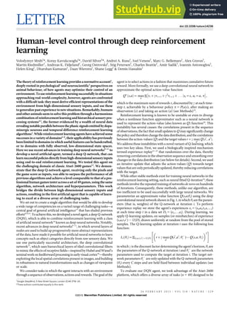
DeepFashion
DeepFashion2
(a)
(b)
tank top
cardigan
tank top
cardigan
vest
vest
skirt
long sleeve
top
long sleeve
outwear
trousers
shorts
shorts
long sleeve
outwear
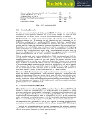
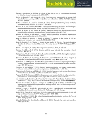
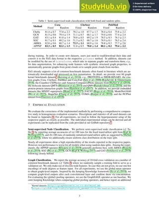
Figure 1. Comparisons between (a) DeepFashion and (b) Deep-
Fashion2. (a) only has single item per image, which is annotated
with 4 ∼ 8 sparse landmarks. The bounding boxes are estimated
from the labeled landmarks, making them noisy. In (b), each im-
age has minimum single item while maximum 7 items. Each item
is manually labeled with bounding box, mask, dense landmarks
(20 per item on average), and commercial-customer image pairs.
challenges can be rooted in the gap between the recent
benchmark and the practical scenario. For example, the
existing largest fashion dataset, DeepFashion [14], has its
own drawbacks such as single clothing item per image,
sparse landmark and pose definition (every clothing cate-
gory shares the same definition of 4 ∼ 8 keypoints), and no
per-pixel mask annotation as shown in Fig.1(a).
To address the above drawbacks, this work presents
DeepFashion2, a large-scale benchmark with comprehen-
sive tasks and annotations of fashion image understanding.
DeepFashion2 contains 491K images of 13 popular cloth-
ing categories. A full spectrum of tasks are defined on
them including clothes detection and recognition, landmark
and pose estimation, segmentation, as well as verification
and retrieval. All these tasks are supported by rich annota-
1
arXiv:1901.07973v1
[cs.CV]
23
Jan
2019](https://image.slidesharecdn.com/5importantdeeplearningresearchpapersyoumustreadin2020-230805220002-b1ad183f/85/5-Important-Deep-Learning-Research-Papers-You-Must-Read-In-2020-17-320.jpg)
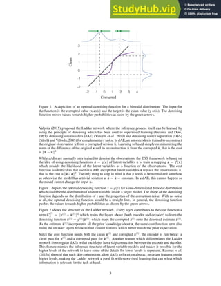
![tions. For instance, DeepFashion2 totally has 801K cloth-
ing items, where each item in an image is labeled with scale,
occlusion, zooming, viewpoint, bounding box, dense land-
marks, and per-pixel mask, as shown in Fig.1(b). These
items can be grouped into 43.8K clothing identities, where
a clothing identity represents the clothes that have almost
the same cutting, pattern, and design. The images of the
same identity are taken by both customers and commercial
shopping stores. An item from the customer and an item
from the commercial store forms a pair. There are 873K
pairs that are 3.5 times larger than DeepFashion. The above
thorough annotations enable developments of strong algo-
rithms to understand fashion images.
This work has three main contributions. (1) We build
a large-scale fashion benchmark with comprehensive tasks
and annotations, to facilitate fashion image analysis. Deep-
Fashion2 possesses the richest definitions of tasks and the
largest number of labels. Its annotations are at least 3.5× of
DeepFashion [14], 6.7× of ModaNet [21], and 8× of Fash-
ionAI [1]. (2) A full spectrum of tasks is carefully defined
on the proposed dataset. For example, to our knowledge,
clothing pose estimation is presented for the first time in the
literature by defining landmarks and poses of 13 categories
that are more diverse and fruitful than human pose. (3) With
DeepFashion2, we extensively evaluate Mask R-CNN [6]
that is a recent advanced framework for visual perception.
A novel Match R-CNN is also proposed to aggregate all the
learned features from clothes categories, poses, and masks
to solve clothing image retrieval in an end-to-end manner.
DeepFashion2 and implementations of Match R-CNN will
be released.
1.1. Related Work
Clothes Datasets. Several clothes datasets have been
proposed such as [20, 5, 7, 14, 21, 1] as summarized in
Table 1. They vary in size as well as amount and type of
annotations. For example, WTBI [5] and DARN [7] have
425K and 182K images respectively. They scraped cat-
egory labels from metadata of the collected images from
online shopping websites, making their labels noisy. In
contrast, CCP [20], DeepFashion [14], and ModaNet [21]
obtain category labels from human annotators. Moreover,
different kinds of annotations are also provided in these
datastes. For example, DeepFashion labels 4∼8 landmarks
(keypoints) per image that are defined on the functional re-
gions of clothes (e.g. ‘collar’). The definitions of these
sparse landmarks are shared across all categories, making
them difficult to capture rich variations of clothing images.
Furthermore, DeepFashion does not have mask annotations.
By comparison, ModaNet [21] has street images with masks
(polygons) of single person but without landmarks. Unlike
existing datasets, DeepFashion2 contains 491K images and
801K instances of landmarks, masks, and bounding boxes,
WTBI
DARN
DeepFashion
ModaNet
FashionAI
DeepFashion2
year 2015[5] 2015[7] 2016[14] 2018[21] 2018[1] now
#images 425K 182K 800K 55K 357K 491K
#categories 11 20 50 13 41 13
#bboxes 39K 7K × × × 801K
#landmarks × × 120K × 100K 801K
#masks × × × 119K × 801K
#pairs 39K 91K 251K × × 873K
Table 1. Comparisons of DeepFashion2 with the other clothes
datasets. The rows represent number of images, bounding boxes,
landmarks, per-pixel masks, and consumer-to-shop pairs respec-
tively. Bounding boxes inferred from other annotations are not
counted.
as well as 873K pairs. It is the most comprehensive bench-
mark of its kinds to date.
Fashion Image Understanding. There are various
tasks that analyze clothing images such as clothes detec-
tion [2, 14], landmark prediction [15, 19, 17], clothes seg-
mentation [18, 20, 13], and retrieval [7, 5, 14]. However,
a unify benchmark and framework to account for all these
tasks is still desired. DeepFashion2 and Match R-CNN fill
in this blank. We report extensive results for the above
tasks with respect to different variations, including scale,
occlusion, zoom-in, and viewpoint. For the task of clothes
retrieval, unlike previous methods [5, 7] that performed
image-level retrieval, DeepFashion2 enables instance-level
retrieval of clothing items. We also present a new fashion
task called clothes pose estimation, which is inspired by
human pose estimation to predict clothing landmarks and
skeletons for 13 clothes categories. This task helps improve
performance of fashion image analysis in real-world appli-
cations.
2. DeepFashion2 Dataset and Benchmark
Overview. DeepFashion2 has four unique characteris-
tics compared to existing fashion datasets. (1) Large Sam-
ple Size. It contains 491K images of 43.8K clothing iden-
tities of interest (unique garment displayed by shopping
stores). On average, each identity has 12.7 items with dif-
ferent styles such as color and printing. DeepFashion2 con-
tained 801K items in total. It is the largest fashion database
to date. Furthermore, each item is associated with various
annotations as introduced above.
(2) Versatility. DeepFashion2 is developed for multiple
tasks of fashion understanding. Its rich annotations support
clothes detection and classification, dense landmark and
pose estimation, instance segmentation, and cross-domain
instance-level clothes retrieval.
(3) Expressivity. This is mainly reflected in two aspects.
First, multiple items are present in a single image, unlike
DeepFashion where each image is labeled with at most one
item. Second, we have 13 different definitions of landmarks
and poses (skeletons) for 13 different categories. There is
2](https://image.slidesharecdn.com/5importantdeeplearningresearchpapersyoumustreadin2020-230805220002-b1ad183f/85/5-Important-Deep-Learning-Research-Papers-You-Must-Read-In-2020-18-320.jpg)
![Short sleeve top
Shorts
Long sleeve dress
Long sleeve outwear
Commercial Customer
(1)
(2)
(3)
Scale
Occlusion
Zoom-in
1
2
3
4
5
6
7
8
9
10
11 12
13
14
15
16
17
18
19
20
21 23
24
25
26
27
28
29
30
31
32 33
34
35
36
37
22
(4)
Viewpoint
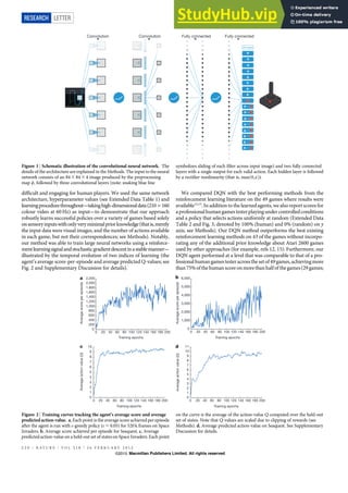
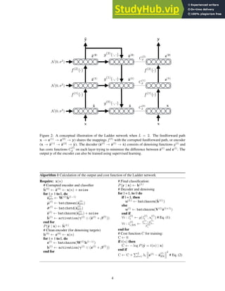
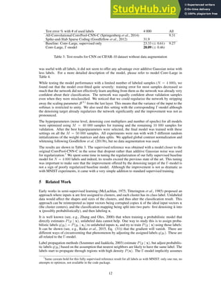
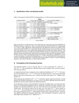
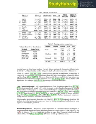
Figure 2. Examples of DeepFashion2. The first column shows definitions of dense landmarks and skeletons of four categories. From (1)
to (4), each row represents clothes images with different variations including ‘scale’, ‘occlusion’, ‘zoom-in’, and ‘viewpoint’. At each row,
we partition the images into two groups, the left three columns represent clothes from commercial stores, while the right three columns are
from customers. In each group, the three images indicate three levels of difficulty with respect to the corresponding variation, including (1)
‘small’, ‘moderate’, ‘large’ scale, (2) ‘slight’, ‘medium’, ‘heavy’ occlusion, (3) ‘no’, ‘medium’, ‘large’ zoom-in, (4) ‘not on human’, ‘side’,
‘back’ viewpoint. Furthermore, at each row, the items in these two groups of images are from the same clothing identity but from two
different domains, that is, commercial and customer. The items of the same identity may have different styles such as color and printing.
Each item is annotated with landmarks and masks.
23 defined landmarks for each category on average. Some
definitions are shown in the first column of Fig.2. These
representations are different from human pose and are not
presented in previous work. They facilitate learning of
strong clothes features that satisfy real-world requirements.
(4) Diversity. We collect data by controlling their vari-
ations in terms of four properties including scale, occlu-
sion, zoom-in, and viewpoint as illustrated in Fig.2, making
DeepFashion2 a challenging benchmark. For each property,
each clothing item is assigned to one of three levels of dif-
ficulty. Fig.2 shows that each identity has high diversity
where its items are from different difficulties.
Data Collection and Cleaning. Raw data of DeepFash-
ion2 are collected from two sources including DeepFashion
[14] and online shopping websites. In particular, images
of each consumer-to-shop pair in DeepFashion are included
in DeepFashion2, while the other images are removed. We
further crawl a large set of images on the Internet from both
commercial shopping stores and consumers. To clean up
the crawled set, we first remove shop images with no corre-
sponding consumer-taken photos. Then human annotators
are asked to clean images that contain clothes with large oc-
clusions, small scales, and low resolutions. Eventually we
have 491K images of 801K items and 873K commercial-
consumer pairs.
Variations. We explain the variations in DeepFashion2.
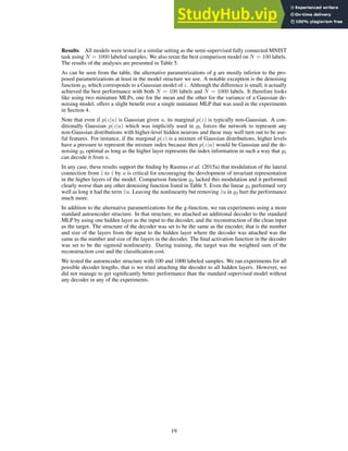
Their statistics are plotted in Fig.3. (1) Scale. We divide all
clothing items into three sets, according to the proportion
of an item compared to the image size, including ‘small’
(< 10%), ‘moderate’ (10% ∼ 40%), and ‘large’ (> 40%).
Fig.3(a) shows that only 50% items have moderate scale.
(2) Occlusion. An item with occlusion means that its re-
gion is occluded by hair, human body, accessory or other
items. Note that an item with its region outside the im-
3](https://image.slidesharecdn.com/5importantdeeplearningresearchpapersyoumustreadin2020-230805220002-b1ad183f/85/5-Important-Deep-Learning-Research-Papers-You-Must-Read-In-2020-19-320.jpg)
![Cardigan Coat Joggers Sweatpants
(a)
(b) (c)
(d)
0
50000
100000
150000
200000
Instance
Number
100
67%
21%
12%
no
medium
large
7%
78%
8%
7% no wear
frontal
side
back
(1) Scale (2) Occlusion (3) Zoom-in (4) Viewpoint
26%
50%
24%
small
moderate
large
47%
47%
6%
slight
medium
heavy
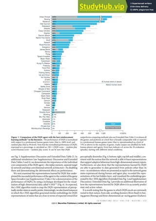
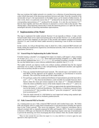
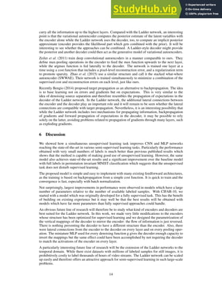
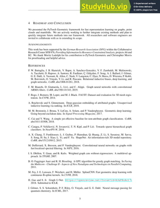
Figure 3. (a) shows the statistics of different variations in DeepFashion2. (b) is the numbers of items of the 13 categories in DeepFashion2.
(c) shows that categories in DeepFashion [14] have ambiguity. For example, it is difficult to distinguish between ‘cardigan’ and ‘coat’, and
between ‘joggers’ and ‘sweatpants’. They result in ambiguity when labeling data. (d) Top: masks may be inaccurate when complex poses
are presented. Bottom: the masks will be refined by human.
age does not belong to this case. Each item is categorized
by the number of its landmarks that are occluded, includ-
ing ‘partial occlusion’(< 20% occluded keypoints), ‘heavy
occlusion’ (> 50% occluded keypoints), ‘medium occlu-
sion’ (otherwise). More than 50% items have medium or
heavy occlusions as summarized in Fig.3. (3) Zoom-in. An
item with zoom-in means that its region is outside the im-
age. This is categorized by the number of landmarks out-
side image. We define ‘no’, ‘large’ (> 30%), and ‘medium’
zoom-in. We see that more than 30% items are zoomed in.
(4) Viewpoint. We divide all items into four partitions in-
cluding 7% clothes that are not on people, 78% clothes on
people from frontal viewpoint, 15% clothes on people from
side or back viewpoint.
2.1. Data Labeling
Category and Bounding Box. Human annotators are
asked to draw a bounding box and assign a category label
for each clothing item. DeepFashion [14] defines 50 cat-
egories but half of them contain less than 5‰ number of
images. Also, ambiguity exists between 50 categories mak-
ing data labeling difficult as shown in Fig.3(c). By grouping
categories in DeepFashion, we derive 13 popular categories
without ambiguity. The numbers of items of 13 categories
are shown in Fig.3(b).
Clothes Landmark, Contour, and Skeleton. As differ-
ent categories of clothes (e.g. upper- and lower-body gar-
ment) have different deformations and appearance changes,
we represent each category by defining its pose, which is a
set of landmarks as well as contours and skeletons between
landmarks. They capture shapes and structures of clothes.
Pose definitions are not presented in previous work and are
significantly different from human pose. For each clothing
item of a category, human annotations are asked to label
landmarks following these instructions.
Moreover, each landmark is assigned one of the two
modes, ‘visible’ or ‘occluded’. We then generate contours
and skeletons automatically by connecting landmarks in a
certain order. To facilitate this process, annotators are also
asked to distinguish landmarks into two types, that is, con-
tour point or junction point. The former one refers to key-
points at the boundary of an item, while the latter one is
assigned to keypoints in conjunction e.g. ‘endpoint of strap
on sling’. The above process controls the labeling quality,
because the generated skeletons help the annotators reex-
amine whether the landmarks are labeled with good quality.
In particular, only when the contour covers the entire item,
the labeled results are eligible, otherwise keypoints will be
refined.
Mask. We label per-pixel mask for each item in a semi-
automatic manner with two stages. The first stage automat-
ically generates masks from the contours. In the second
stage, human annotators are asked to refine the masks, be-
cause the generated masks may be not accurate when com-
plex human poses are presented. As shown in Fig.3(d), the
mark is inaccurate when an image is taken from side-view
of people crossing legs. The masks will be refined by hu-
man.
Style. As introduced before, we collect 43.8K different
clothing identities where each identity has 13 items on av-
erage. These items are further labeled with different styles
such as color, printing, and logo. Fig.2 shows that a pair
of clothes that have the same identity could have different
styles.
2.2. Benchmarks
We build four benchmarks by using the images and la-
bels from DeepFashion2. For each benchmark, there are
4](https://image.slidesharecdn.com/5importantdeeplearningresearchpapersyoumustreadin2020-230805220002-b1ad183f/85/5-Important-Deep-Learning-Research-Papers-You-Must-Read-In-2020-20-320.jpg)
![391K images for training, 34K images for validation and
67K images for test.
Clothes Detection. This task detects clothes in an im-
age by predicting bounding boxes and category labels. The
evaluation metrics are the bounding box’s average preci-
sion APbox, APIoU=0.50
box , and APIoU=0.75
box by following
COCO [11].
Landmark Estimation. This task aims to predict land-
marks for each detected clothing item in an each image.
Similarly, we employ the evaluation metrics used by COCO
for human pose estimation by calculating the average pre-
cision for keypoints APpt, APOKS=0.50
pt , and APOKS=0.75
pt ,
where OKS indicates the object landmark similarity.
Segmentation. This task assigns a category label
(including background label) to each pixel in an item.
The evaluation metrics is the average precision includ-
ing APmask, APIoU=0.50
mask , and APIoU=0.75
mask computed over
masks.
Commercial-Consumer Clothes Retrieval. Given a
detected item from a consumer-taken photo, this task aims
to search the commercial images in the gallery for the items
that are corresponding to this detected item. This setting
is more realistic than DeepFashion [14], which assumes
ground-truth bounding box is provided. In this task, top-k
retrieval accuracy is employed as the evaluation metric. We
emphasize the retrieval performance while still consider the
influence of detector. If a clothing item fails to be detected,
this query item is counted as missed. In particular, we have
more than 686K commercial-consumer clothes pairs in the
training set. In the validation set, there are 10, 990 con-
sumer images with 12, 550 items as a query set, and 21, 438
commercial images with 37, 183 items as a gallery set. In
the test set, there are 21, 550 consumer images with 24, 402
items as queries, while 43, 608 commercial images with
75, 347 items in the gallery.
3. Match R-CNN
We present a strong baseline model built upon Mask R-
CNN [6] for DeepFashion2, termed Match R-CNN, which
is an end-to-end training framework that jointly learns
clothes detection, landmark estimation, instance segmenta-
tion, and consumer-to-shop retrieval. The above tasks are
solved by using different streams and stacking a Siamese
module on top of these streams to aggregate learned fea-
tures.
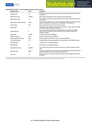
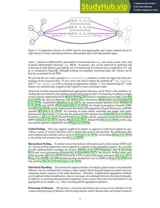
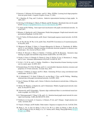
As shown in Fig.4, Match R-CNN employs two images
I1 and I2 as inputs. Each image is passed through three
main components including a Feature Network (FN), a Per-
ception Network (PN), and a Matching Network (MN). In
the first stage, FN contains a ResNet-FPN [10] backbone,
a region proposal network (RPN) [16] and RoIAlign mod-
ule. An image is first fed into ResNet50 to extract features,
which are then fed into a FPN that uses a top-down architec-
ResNet
FPN
7x7x
256 1024
class
box
1024
RoIAlign
14x14
x256
RoIAlign
RoIAlign
14x14
x256
28x28
x256 mask
14x14
x256
14x14
x512
28x28
x32
landmark
NxN
x256
1024
NxNx
1024
matching score
256
z
256
Sub Square FC
not matching score
FN
𝐼"
𝐼#
FN PN
PN
NxN
x256
1024
NxNx
1024
𝐼"
MN
𝑣"
𝑣#
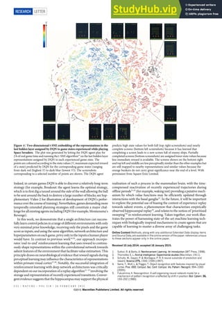
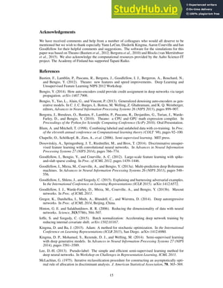
Figure 4. Diagram of Match R-CNN that contains three main
components including a feature extraction network (FN), a per-
ception network (PN), and a match network (MN).
ture with lateral connections to build a pyramid of feature
maps. RoIAlign extracts features from different levels of
the pyramid map.
In the second stage, PN contains three streams of net-
works including landmark estimation, clothes detection,
and mask prediction as shown in Fig.4. The extracted RoI
features after the first stage are fed into three streams in
PN separately. The clothes detection stream has two hidden
fully-connected (fc) layers, one fc layer for classification,
and one fc layer for bounding box regression. The stream of
landmark estimation has 8 ‘conv’ layers and 2 ‘deconv’ lay-
ers to predict landmarks. Segmentation stream has 4 ‘conv’
layers, 1 ‘deconv’ layer, and another ‘conv’ layer to predict
masks.
In the third stage, MN contains a feature extractor and
a similarity learning network for clothes retrieval. The
learned RoI features after the FN component are highly
discriminative with respect to clothes category, pose, and
mask. They are fed into MN to obtain features vectors
for retrieval, where v1 and v2 are passed into the similar-
ity learning network to obtain the similarity score between
the detected clothing items in I1 and I2. Specifically, the
feature extractor has 4 ‘conv’ layers, one pooling layer, and
one fc layer. The similarity learning network consists of
subtraction and square operator and a fc layer, which esti-
mates the probability of whether two clothing items match
or not.
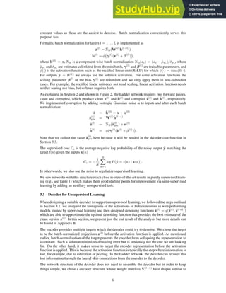
Loss Functions. The parameters Θ of the Match R-CNN
are optimized by minimizing five loss functions, which are
formulated as minΘ L = λ1Lcls + λ2Lbox + λ3Lpose +
λ4Lmask + λ5Lpair, including a cross-entropy (CE) loss
Lcls for clothes classification, a smooth loss [4] Lbox for
bounding box regression, a CE loss Lpose for landmark es-
5](https://image.slidesharecdn.com/5importantdeeplearningresearchpapersyoumustreadin2020-230805220002-b1ad183f/85/5-Important-Deep-Learning-Research-Papers-You-Must-Read-In-2020-21-320.jpg)
![scale occlusion zoom-in viewpoint overall
small moderate large slight medium heavy no medium large no wear frontal side or back
APbox 0.604 0.700 0.660 0.712 0.654 0.372 0.695 0.629 0.466 0.624 0.681 0.641 0.667
APIoU=0.50
box 0.780 0.851 0.768 0.844 0.810 0.531 0.848 0.755 0.563 0.713 0.832 0.796 0.814
APIoU=0.75
box 0.717 0.809 0.744 0.812 0.768 0.433 0.806 0.718 0.525 0.688 0.791 0.744 0.773
Table 2. Clothes detection of Mask R-CNN [6] on different validation subsets, including scale, occlusion, zoom-in, and viewpoint. The
evaluation metrics are APbox, APIoU=0.50
box , and APIoU=0.75
box . The best performance of each subset is bold.
long sleeve dress 0.80
(a)
(b)
short sleeve dress
long sleeve outwear
long sleeve dress
shorts
long sleeve top
long sleeve outwear
vest
outwear sling
skirt vest dress
vest
long sleeve top
Figure 5. (a) shows failure cases in clothes detection while (b) shows failure cases in clothes segmentation. In (a) and (b), the missing
bounding boxes are drawn in red while the correct category labels are also in red. Inaccurate masks are also highlighted by arrows in (b).
For example, clothes fail to be detected or segmented in too small scale, too large scale, large non-rigid deformation, heavy occlusion, large
zoom-in, side or back viewpoint.
timation, a CE loss Lmask for clothes segmentation, and a
CE loss Lpair for clothes retrieval. Specifically, Lcls, Lbox,
Lpose, and Lmask are identical as defined in [6]. We have
Lpair = − 1
n
Pn
i=1[yilog(ŷi) + (1 − yi)log(1 − ŷi)], where
yi = 1 indicates the two items of a pair are matched, other-
wise yi = 0.
Implementations. In our experiments, each training im-
age is resized to its shorter edge of 800 pixels with its longer
edge that is no more than 1333 pixels. Each minibatch has
two images in a GPU and 8 GPUs are used for training.
For minibatch size 16, the learning rate (LR) schedule starts
at 0.02 and is decreased by a factor of 0.1 after 8 epochs
and then 11 epochs, and finally terminates at 12 epochs.
This scheduler is denoted as 1x. Mask R-CNN adopts 2x
schedule for clothes detection and segmentation where ‘2x’
is twice as long as 1x with the LR scaled proportionally.
Then It adopts s1x for landmark and pose estimation where
s1x scales the 1x schedule by roughly 1.44x. Match R-
CNN uses 1x schedule for consumer-to-shop clothes re-
trieval. The above models are trained by using SGD with
a weight decay of 10−5
and momentum of 0.9.
In our experiments, the RPN produces anchors with 3 as-
pect rations on each level of the FPN pyramid. In clothes
detection stream, an RoI is considered positive if its IoU
with a ground truth box is larger than 0.5 and negative oth-
erwise. In clothes segmentation stream, positive RoIs with
foreground label are chosen while in landmark estimation
stream, positive RoIs with visible landmarks are selected.
We define ground truth box of interest as clothing items
whose style number is > 0 and can constitute matching
pairs. In clothes retrieval stream, RoIs are selected if their
IoU with a ground truth box of interest is larger than 0.7. If
RoI features are extracted from landmark estimation stream,
RoIs with visible landmarks are also selected.
Inference. At testing time, images are resized in the
same way as the training stage. The top 1000 proposals with
detection probabilities are chosen for bounding box classi-
fication and regression. Then non-maximum suppression is
applied to these proposals. The filtered proposals are fed
into the landmark branch and the mask branch separately.
For the retrieval task, each unique detected clothing item in
consumer-taken image with highest confidence is selected
as query.
4. Experiments
We demonstrate the effectiveness of DeepFashion2 by
evaluating Mask R-CNN [6] and Match R-CNN in multiple
tasks including clothes detection and classification, land-
mark estimation, instance segmentation, and consumer-to-
6](https://image.slidesharecdn.com/5importantdeeplearningresearchpapersyoumustreadin2020-230805220002-b1ad183f/85/5-Important-Deep-Learning-Research-Papers-You-Must-Read-In-2020-22-320.jpg)
![scale occlusion zoom-in viewpoint overall
small moderate large slight medium heavy no medium large no wear frontal side or back
APpt
0.587 0.687 0.599 0.669 0.631 0.398 0.688 0.559 0.375 0.527 0.677 0.536 0.641
0.497 0.607 0.555 0.643 0.530 0.248 0.616 0.489 0.319 0.510 0.596 0.456 0.563
APOKS=0.50
pt
0.780 0.854 0.782 0.851 0.813 0.534 0.855 0.757 0.571 0.724 0.846 0.748 0.820
0.764 0.839 0.774 0.847 0.799 0.479 0.848 0.744 0.549 0.716 0.832 0.727 0.805
APOKS=0.75
pt
0.671 0.779 0.678 0.760 0.718 0.440 0.786 0.633 0.390 0.571 0.771 0.610 0.728
0.551 0.703 0.625 0.739 0.600 0.236 0.714 0.537 0.307 0.550 0.684 0.506 0.641
Table 3. Landmark estimation of Mask R-CNN [6] on different validation subsets, including scale, occlusion, zoom-in, and viewpoint.
Results of evaluation on visible landmarks only and evaluation on both visible and occlusion landmarks are separately shown in each row.
The evaluation metrics are APpt, APOKS=0.50
pt , and APOKS=0.75
pt . The best performance of each subset is bold.
(b)
(c)
(d)
(1) (2)
0
0.2
0.4
0.6
1 5 10 15 20
Retrieval
Accuracy
Retrieved Instance
class pose mask
pose+class mask+class
0
0.2
0.4
0.6
1 5 10 15 20
Retrieval
Accuracy
Retrieved Instance
class pose mask
pose+class mask+class
(a)
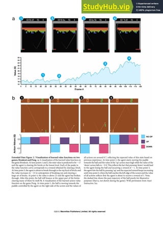
Figure 6. (a) shows results of landmark and pose estimation. (b)
shows results of clothes segmentation. (c) shows queries with top-
5 retrieved clothing items. The first column is the image from the
customer with bounding box predicted by detection module, and
the second to the sixth columns show the retrieval results from the
store. (d) is the retrieval accuracy of overall query validation set
with (1) detected box (2) ground truth box. Evaluation metrics are
top-1, -5, -10, -15, and -20 retrieval accuracy.
shop clothes retrieval. To further show the large variations
of DeepFashion2, the validation set is divided into three
subsets according to their difficulty levels in scale, occlu-
sion, zoom-in, and viewpoint. The settings of Mask R-CNN
and Match R-CNN follow Sec.3. All models are trained in
the training set and evaluated in the validation set.
The following sections from 4.1 to 4.4 report results for
different tasks, showing that DeepFashion2 imposes signif-
icant challenges to both Mask R-CNN and Match R-CNN,
which are the recent state-of-the-art systems for visual per-
ception.
4.1. Clothes Detection
Table 2 summarizes the results of clothes detection on
different difficulty subsets. We see that the clothes of mod-
erate scale, slight occlusion, no zoom-in, and frontal view-
point have the highest detection rates. There are several
observations. First, detecting clothes with small or large
scale reduces detection rates. Some failure cases are pro-
vided in Fig.5(a) where the item could occupy less than 2%
of the image while some occupies more than 90% of the
image. Second, in Table 2, it is intuitively to see that heavy
occlusion and large zoom-in degenerate performance. In
these two cases, large portions of the clothes are invisible
as shown in Fig.5(a). Third, it is seen in Table 2 that the
clothing items not on human body also drop performance.
This is because they possess large non-rigid deformations as
visualized in the failure cases of Fig.5(a). These variations
are not presented in previous object detection benchmarks
such as COCO. Fourth, clothes with side or back viewpoint,
are much more difficult to detect as shown in Fig.5(a).
4.2. Landmark and Pose Estimation
Table 3 summarizes the results of landmark estimation.
The evaluation of each subset is performed in two settings,
including visible landmark only (the occluded landmarks
are not evaluated), as well as both visible and occluded
landmarks. As estimating the occluded landmarks is more
difficult than visible landmarks, the second setting generally
provides worse results than the first setting.
In general, we see that Mask R-CNN obtains an overall
7](https://image.slidesharecdn.com/5importantdeeplearningresearchpapersyoumustreadin2020-230805220002-b1ad183f/85/5-Important-Deep-Learning-Research-Papers-You-Must-Read-In-2020-23-320.jpg)
![scale occlusion zoom-in viewpoint overall
small moderate large slight medium heavy no medium large no wear frontal side or back
APmask 0.634 0.700 0.669 0.720 0.674 0.389 0.703 0.627 0.526 0.695 0.697 0.617 0.680
APIoU=0.50
mask 0.831 0.900 0.844 0.900 0.878 0.559 0.899 0.815 0.663 0.829 0.886 0.843 0.873
APIoU=0.75
mask 0.765 0.838 0.786 0.850 0.813 0.463 0.842 0.740 0.613 0.792 0.834 0.732 0.812
Table 4. Clothes segmentation of Mask R-CNN [6] on different validation subsets, including scale, occlusion, zoom-in, and viewpoint.
The evaluation metrics are APmask, APIoU=0.50
mask , and APIoU=0.75
mask . The best performance of each subset is bold.
scale occlusion zoom-in viewpoint overall
small moderate large slight medium heavy no medium large no wear frontal side or back top-1 top-10 top-20
class
0.513 0.619 0.547 0.580 0.556 0.503 0.608 0.557 0.441 0.555 0.580 0.533 0.122 0.363 0.464
0.445 0.558 0.515 0.542 0.514 0.361 0.557 0.514 0.409 0.508 0.529 0.519 0.104 0.321 0.417
pose
0.695 0.775 0.729 0.752 0.729 0.698 0.769 0.742 0.618 0.725 0.755 0.705 0.255 0.555 0.647
0.619 0.695 0.688 0.704 0.668 0.559 0.700 0.693 0.572 0.682 0.690 0.654 0.234 0.495 0.589
mask
0.641 0.705 0.663 0.688 0.656 0.645 0.708 0.670 0.556 0.650 0.690 0.653 0.187 0.471 0.573
0.584 0.656 0.632 0.657 0.619 0.512 0.663 0.630 0.541 0.628 0.645 0.602 0.175 0.421 0.529
pose+class
0.752 0.786 0.733 0.754 0.750 0.728 0.789 0.750 0.620 0.726 0.771 0.719 0.268 0.574 0.665
0.691 0.730 0.705 0.725 0.706 0.605 0.746 0.709 0.582 0.699 0.723 0.684 0.244 0.522 0.617
mask+class
0.679 0.738 0.685 0.711 0.695 0.651 0.742 0.699 0.569 0.677 0.719 0.678 0.214 0.510 0.607
0.623 0.696 0.661 0.685 0.659 0.568 0.708 0.667 0.566 0.659 0.676 0.657 0.200 0.463 0.564
Table 5. Consumer-to-Shop Clothes Retrieval of Match R-CNN on different subsets of some validation consumer-taken images. Each
query item in these images has over 5 identical clothing items in validation commercial images. Results of evaluation on ground truth box
and detected box are separately shown in each row. The evaluation metrics are top-20 accuracy. The best performance of each subset is
bold.
AP of just 0.563, showing that clothes landmark estimation
could be even more challenging than human pose estima-
tion in COCO. In particular, Table 3 exhibits similar trends
as those from clothes detection. For example, the cloth-
ing items with moderate scale, slight occlusion, no zoom-
in, and frontal viewpoint have better results than the others
subsets. Moreover, heavy occlusion and zoom-in decreases
performance a lot. Some results are given in Fig.6(a).
4.3. Clothes Segmentation
Table 4 summarizes the results of segmentation. The
performance declines when segmenting clothing items with
small and large scale, heavy occlusion, large zoom-in, side
or back viewpoint, which is consistent with those trends in
the previous tasks. Some results are given in Fig.6(b). Some
failure cases are visualized in Fig.5(b).
4.4. Consumer-to-Shop Clothes Retrieval
Table 5 summarizes the results of clothes retrieval. The
retrieval accuracy is reported in Fig. 6(d), where top-1, -
5, -10, and -20 retrieval accuracy are shown. We evaluate
two settings in (c.1) and (c.2), when the bounding boxes
are predicted by the detection module in Match R-CNN and
are provided as ground truths. Match R-CNN achieves a
top-20 accuracy of less than 0.7 with ground-truth bounding
boxes provided, indicating that the retrieval benchmark is
challenging. Furthermore, retrieval accuracy drops when
using detected boxes, meaning that this is a more realistic
setting.
In Table 5, different combinations of the learned features
are also evaluated. In general, the combination of features
increases the accuracy. In particular, the learned features
from pose and class achieve better results than the other
features. When comparing learned features from pose and
mask, we find that the former achieves better results, indi-
cating that landmark locations can be more robust across
scenarios.
As shown in Table 5, the performance declines when
small scale, heavily occluded clothing items are presented.
Clothes with large zoom-in achieved the lowest accuracy
because only part of clothes are displayed in the image and
crucial distinguishable features may be missing. Compared
with clothes on people from frontal view, clothes from side
or back viewpoint perform worse due to lack of discrim-
inative features like patterns on the front of tops. Exam-
ple queries with top-5 retrieved clothing items are shown in
Fig.6(c).
5. Conclusions
This work represented DeepFashion2, a large-scale fash-
ion image benchmark with comprehensive tasks and an-
notations. DeepFashion2 contains 491K images, each of
which is richly labeled with style, scale, occlusion, zoom-
ing, viewpoint, bounding box, dense landmarks and pose,
pixel-level masks, and pair of images of identical item from
consumer and commercial store. We establish benchmarks
covering multiple tasks in fashion understanding, including
clothes detection, landmark and pose estimation, clothes
segmentation, consumer-to-shop verification and retrieval.
A novel Match R-CNN framework that builds upon Mask
R-CNN is proposed to solve the above tasks in end-to-end
manner. Extensive evaluations are conducted in DeepFash-
8](https://image.slidesharecdn.com/5importantdeeplearningresearchpapersyoumustreadin2020-230805220002-b1ad183f/85/5-Important-Deep-Learning-Research-Papers-You-Must-Read-In-2020-24-320.jpg)
![ion2.
The rich data and labels of DeepFashion2 will defi-
nitely facilitate the developments of algorithms to under-
stand fashion images in future work. We will focus on
three aspects. First, more challenging tasks will be explored
with DeepFashion2, such as synthesizing clothing images
by using GANs. Second, it is also interesting to explore
multi-domain learning for clothing images, because fashion
trends of clothes may change frequently, making variations
of clothing images changed. Third, we will introduce more
evaluation metrics into DeepFashion2, such as size, run-
time, and memory consumptions of deep models, towards
understanding fashion images in real-world scenario.
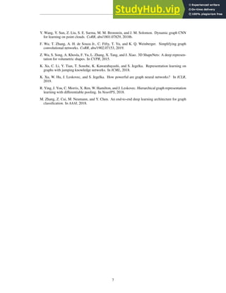
References
[1] Fashionai dataset. http://fashionai.alibaba.
com/datasets/.
[2] H. Chen, A. Gallagher, and B. Girod. Describing clothing by
semantic attributes. In ECCV, 2012.
[3] Q. Chen, J. Huang, R. Feris, L. M. Brown, J. Dong, and
S. Yan. Deep domain adaptation for describing people based
on fine-grained clothing attributes. In CVPR, 2015.
[4] R. Girshick. Fast r-cnn. In ICCV, 2015.
[5] M. Hadi Kiapour, X. Han, S. Lazebnik, A. C. Berg, and T. L.
Berg. Where to buy it: Matching street clothing photos in
online shops. In ICCV, 2015.
[6] K. He, G. Gkioxari, P. Dollár, and R. Girshick. Mask r-cnn.
In ICCV, 2017.
[7] J. Huang, R. S. Feris, Q. Chen, and S. Yan. Cross-domain
image retrieval with a dual attribute-aware ranking network.
In ICCV, 2015.
[8] X. Ji, W. Wang, M. Zhang, and Y. Yang. Cross-domain image
retrieval with attention modeling. In ACM Multimedia, 2017.
[9] L. Liao, X. He, B. Zhao, C.-W. Ngo, and T.-S. Chua. Inter-
pretable multimodal retrieval for fashion products. In ACM
Multimedia, 2018.
[10] T.-Y. Lin, P. Dollár, R. B. Girshick, K. He, B. Hariharan, and
S. J. Belongie. Feature pyramid networks for object detec-
tion. In CVPR, 2017.
[11] T.-Y. Lin, M. Maire, S. Belongie, J. Hays, P. Perona, D. Ra-
manan, P. Dollár, and C. L. Zitnick. Microsoft coco: Com-
mon objects in context. In ECCV, 2014.
[12] K.-H. Liu, T.-Y. Chen, and C.-S. Chen. Mvc: A dataset for
view-invariant clothing retrieval and attribute prediction. In
ACM Multimedia, 2016.
[13] S. Liu, X. Liang, L. Liu, K. Lu, L. Lin, X. Cao, and S. Yan.
Fashion parsing with video context. IEEE Transactions on
Multimedia, 17(8):1347–1358, 2015.
[14] Z. Liu, P. Luo, S. Qiu, X. Wang, and X. Tang. Deepfashion:
Powering robust clothes recognition and retrieval with rich
annotations. In CVPR, 2016.
[15] Z. Liu, S. Yan, P. Luo, X. Wang, and X. Tang. Fashion land-
mark detection in the wild. In ECCV, 2016.
[16] S. Ren, K. He, R. Girshick, and J. Sun. Faster r-cnn: Towards
real-time object detection with region proposal networks. In
NIPS, 2015.
[17] W. Wang, Y. Xu, J. Shen, and S.-C. Zhu. Attentive fashion
grammar network for fashion landmark detection and cloth-
ing category classification. In CVPR, 2018.
[18] K. Yamaguchi, M. Hadi Kiapour, and T. L. Berg. Paper doll
parsing: Retrieving similar styles to parse clothing items. In
ICCV, 2013.
[19] S. Yan, Z. Liu, P. Luo, S. Qiu, X. Wang, and X. Tang. Un-
constrained fashion landmark detection via hierarchical re-
current transformer networks. In ACM Multimedia, 2017.
[20] W. Yang, P. Luo, and L. Lin. Clothing co-parsing by joint
image segmentation and labeling. In CVPR, 2014.
[21] S. Zheng, F. Yang, M. H. Kiapour, and R. Piramuthu.
Modanet: A large-scale street fashion dataset with polygon
annotations. In ACM Multimedia, 2018.
9](https://image.slidesharecdn.com/5importantdeeplearningresearchpapersyoumustreadin2020-230805220002-b1ad183f/85/5-Important-Deep-Learning-Research-Papers-You-Must-Read-In-2020-25-320.jpg)
![Semi-Supervised Learning with Ladder Network
Antti Rasmus
Nvidia, Finland
Harri Valpola
ZenRobotics, Finland
Mikko Honkala
Nokia Technologies, Finland
Mathias Berglund
Aalto University, Finland
Tapani Raiko
Aalto University, Finland
Abstract
We combine supervised learning with unsupervised learning in deep neural net-
works. The proposed model is trained to simultaneously minimize the sum of su-
pervised and unsupervised cost functions by backpropagation, avoiding the need
for layer-wise pretraining. Our work builds on top of the Ladder network pro-
posed by Valpola (2015) which we extend by combining the model with super-
vision. We show that the resulting model reaches state-of-the-art performance in
various tasks: MNIST and CIFAR-10 classification in a semi-supervised setting
and permutation invariant MNIST in both semi-supervised and full-labels setting.
1 Introduction
In this paper, we introduce an unsupervised learning method that fits well with supervised learning.
The idea of using unsupervised learning to complement supervision is not new. Combining an
auxiliary task to help train a neural network was proposed by Suddarth and Kergosien (1990). By
sharing the hidden representations among more than one task, the network generalizes better. There
are multiple choices for the unsupervised task, for example, reconstructing the inputs at every level
of the model (e.g., Ranzato and Szummer, 2008) or classification of each input sample into its own
class (Dosovitskiy et al., 2014).
Although some methods have been able to simultaneously apply both supervised and unsupervised
learning (Ranzato and Szummer, 2008; Goodfellow et al., 2013a), often these unsupervised auxil-
iary tasks are only applied as pre-training, followed by normal supervised learning (e.g., Hinton and
Salakhutdinov, 2006). In complex tasks there is often much more structure in the inputs than can
be represented, and unsupervised learning cannot, by definition, know what will be useful for the
task at hand. Consider, for instance, the autoencoder approach applied to natural images: an aux-
iliary decoder network tries to reconstruct the original input from the internal representation. The
autoencoder will try to preserve all the details needed for reconstructing the image at pixel level,
even though classification is typically invariant to all kinds of transformations which do not preserve
pixel values. Most of the information required for pixel-level reconstruction is irrelevant and takes
space from the more relevant invariant features which, almost by definition, cannot alone be used
for reconstruction.
Our approach follows Valpola (2015) who proposed a Ladder network where the auxiliary task is
to denoise representations at every level of the model. The model structure is an autoencoder with
skip connections from the encoder to decoder and the learning task is similar to that in denoising
autoencoders but applied to every layer, not just inputs. The skip connections relieve the pressure to
represent details at the higher layers of the model because, through the skip connections, the decoder
can recover any details discarded by the encoder. Previously the Ladder network has only been
demonstrated in unsupervised learning (Valpola, 2015; Rasmus et al., 2015a) but we now combine
it with supervised learning.
1
arXiv:1507.02672v1
[cs.NE]
9
Jul
2015](https://image.slidesharecdn.com/5importantdeeplearningresearchpapersyoumustreadin2020-230805220002-b1ad183f/85/5-Important-Deep-Learning-Research-Papers-You-Must-Read-In-2020-26-320.jpg)
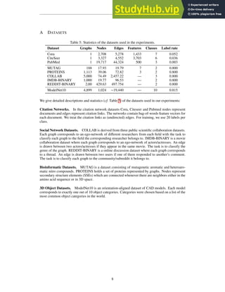
![Figure 3: Each hidden neuron is denoised using a miniature MLP network with two inputs, ui and
z̃i and a single output ẑi. The network has a single sigmoidal unit, skip connections from input to
output and input augmented by the product uiẑi. The total number of parameters is therefore 9 per
each hidden neuron
the weight matrices W(l)
of the encoder, except being transposed, and which performs the denois-
ing neuron-wise. This keeps the number of parameters of the decoder in check but still allows the
network to represent any distributions: any dependencies between hidden neurons can still be repre-
sented through the higher levels of the network which effectively implement a higher-level denoising
autoencoder.
In practice the neuron-wise denoising function g is implemented by first computing a vertical map-
ping from ẑ(l+1)
and then batch normalizing the resulting projections:
u(l)
= NB(V(l+1)
ẑ(l+1)
) ,
where the matrix V(l)
has the same dimension as the transpose of W(l)
on the encoder side. The
projection vector u(l)
has the same dimensionality as z(l)
which means that the final denoising can
be applied neuro-wise with a miniature MLP network that takes two inputs, z̃
(l)
i and u
(l)
i , and outputs
the denoised estimate ẑ
(l)
i :
ẑ
(l)
i = g
(l)
i (z̃
(l)
i , u
(l)
i ) .
Note the slight abuse of notation here since g
(l)
i is now a function of scalars z̃
(l)
i and u
(l)
i rather than
the full vectors z̃(l)
and ẑ(l+1)
.
Figure 3 illustrates the structure of the miniature MLPs which are parametrized as follows:
ẑ
(l)
i = g
(l)
i (z̃
(l)
i , u
(l)
i ) = a
(l)
i ξ
(l)
i + b
(l)
i sigmoid(c
(l)
i ξ
(l)
i ) (1)
where ξ
(l)
i = [1, z̃
(l)
i , u
(l)
i , z̃
(l)
i u
(l)
i ]T
is the augmented input, a
(l)
i and c
(l)
i are trainable 1 × 4 weight
vectors, and b
(l)
i is a trainable weight. In other words, each hidden neuron of the network has its
own miniature MLP network with 9 parameters. While this makes the number of parameters in the
decoder slightly higher than in the encoder, the difference is insignificant as most of the parameters
are in the vertical projection mappings W(l)
and V(l)
which have the same dimensions (apart from
transposition).
For the lowest layer, x̂ = ẑ(0)
and x̃ = z̃(0)
by definition, and for the highest layer we chose
u(L)
= ỹ. This allows the highest-layer denoising function to utilize prior information about the
classes being mutually exclusive which seems to improve convergence in cases where there are very
few labeled samples.
The proposed parametrization is capable of learning denoising of several different distributions in-
cluding sub- and super-Gaussian and bimodal distributions. This means that the decoder supports
sparse coding and independent component analysis.3
The parametrization also allows the distribu-
tion to be modulated by z(l+1)
through u(l)
, encouraging the decoder to find representations z(l)
that
3
For more details on how denoising functions represent corresponding distributions see Valpola (2015,
Section 4.1).
7](https://image.slidesharecdn.com/5importantdeeplearningresearchpapersyoumustreadin2020-230805220002-b1ad183f/85/5-Important-Deep-Learning-Research-Papers-You-Must-Read-In-2020-32-320.jpg)
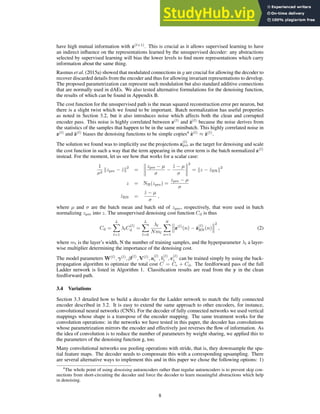

![Based on this analysis, we proposed the following parametrization for g:
ẑ = g(z̃, u) = aξ + bsigmoid(cξ) (3)
where ξ = [1, z̃, u, z̃u]T
is the augmented input, a and c are trainable weight vectors, b is a train-
able scalar weight. We have left out the superscript (l) and subscript i in order not to clutter the
equations8
. This corresponds to a miniature MLP network as explained in Section 3.3.
In order to test whether the elements of the proposed function g were necessary, we systematically
removed components from g or changed g altogether and compared to the results obtained with the
original parametrization. We tuned the hyperparameters of each comparison model separately using
a grid search over some of the relevant hyperparameters. However, the std of additive Gaussian
corruption noise was set to 0.3. This means that with N = 1000 labels, the comparison does not
include the best-performing model reported in Table 1.
As in the proposed function g, all comparison denoising functions mapped neuron-wise the cor-
rupted hidden layer pre-activation z̃(l)
to the reconstructed hidden layer activation given one projec-
tion from the reconstruction of the layer above: ẑ
(l)
i = g(z̃
(l)
i , u
(l)
i ).
Test error % with # of used labels 100 1000
Proposed function g: miniature MLP with z̃u 1.11 (± 0.07) 1.11 (± 0.06)
Comparison g2: No augmented term z̃u 2.03 (± 0.09) 1.70 (± 0.08)
Comparison g3: Linear g but with z̃u 1.49 (± 0.10) 1.30 (± 0.08)
Comparison g4: Only the mean depends on u 2.90 (± 1.19) 2.11 (± 0.45)
Comparison g5: Gaussian z 1.06 (± 0.07) 1.03 (± 0.06)
Table 5: Semi-supervised results from the MNIST dataset. The proposed function g is compared to
alternative parametrizations
The comparison functions g2...5 are parametrized as follows:
Comparison g2: No augmented term
g2(z̃, u) = aξ′
+ bsigmoid(cξ′
) (4)
where ξ′
= [1, z̃, u]T
. g2 therefore differs from g in that the input lacks the augmented term z̃u. In
the original formulation, the augmented term was expected to increase the freedom of the denoising
to modulate the distribution of z by u. However, we wanted to test the effect on the results.
Comparison g3: Linear g
g3(z̃, u) = aξ. (5)
g3 differs from g in that it is linear and does not have a sigmoid term. As this formulation is linear,
it only supports Gaussian distributions. Although the parametrization has the augmented term that
lets u modulate the slope and shift of the distribution, the scope of possible denoising functions is
still fairly limited.
Comparison g4: u affects only the mean of p(z | u)
g4(z̃, u) = a1u + a2sigmoid(a3u + a4) + a5z̃ + a6sigmoid(a7z̃ + a8) + a9 (6)
g4 differs from g in that the inputs from u are not allowed to modulate the terms that depend on z̃,
but that the effect is additive. This means that the parametrization only supports optimal denoising
functions for a conditional distribution p(z | u) where u only shifts the mean of the distribution of z
but otherwise leaves the shape of the distribution intact.
Comparison g5: Gaussian z As reviewed by Valpola (2015, Section 4.1), assuming z is Gaussian
given u, the optimal denoising can be represented as
g5(z̃, u) = (z̃ − µ(u)) υ(u) + µ(u) . (7)
We modeled both µ(u) and υ(u) with a miniature MLP network: µ(u) = a1sigmoid(a2u + a3) +
a4u + a5 and υ(u) = a6sigmoid(a7u + a8) + a9u + a10. Given u, this parametrization is linear
with respect to z̃, and both the slope and the bias depended nonlinearly on u.
8
For the exact definition, see Eq. (1).
18](https://image.slidesharecdn.com/5importantdeeplearningresearchpapersyoumustreadin2020-230805220002-b1ad183f/85/5-Important-Deep-Learning-Research-Papers-You-Must-Read-In-2020-43-320.jpg)
![FAST GRAPH REPRESENTATION LEARNING WITH
PYTORCH GEOMETRIC
Matthias Fey Jan E. Lenssen
Department of Computer Graphics
TU Dortmund University
44227 Dortmund, Germany
{matthias.fey,janeric.lenssen}@udo.edu
ABSTRACT
We introduce PyTorch Geometric, a library for deep learning on irregularly struc-
tured input data such as graphs, point clouds and manifolds, built upon PyTorch. In
addition to general graph data structures and processing methods, it contains a va-
riety of recently published methods from the domains of relational learning and 3D
data processing. PyTorch Geometric achieves high data throughput by leveraging
sparse GPU acceleration, by providing dedicated CUDA kernels and by introduc-
ing efficient mini-batch handling for input examples of different size. In this work,
we present the library in detail and perform a comprehensive comparative study of
the implemented methods in homogeneous evaluation scenarios.
1 INTRODUCTION
Graph Neural Networks (GNNs) recently emerged as a powerful approach for representation learning
on graphs, point clouds and manifolds (Bronstein et al., 2017; Kipf Welling, 2017). Similar to the
concepts of convolutional and pooling layers on regular domains, GNNs are able to (hierarchically)
extract localized embeddings by passing, transforming, and aggregating information (Bronstein et al.,
2017; Gilmer et al., 2017; Battaglia et al., 2018; Ying et al., 2018).
However, implementing GNNs is challenging, as high GPU throughput needs to be achieved on
highly sparse and irregular data of varying size. Here, we introduce PyTorch Geometric (PyG), a
geometric deep learning extension library for PyTorch (Paszke et al., 2017) which achieves high
performance by leveraging dedicated CUDA kernels. Following a simple message passing API, it
bundles most of the recently proposed convolutional and pooling layers into a single and unified
framework. All implemented methods support both CPU and GPU computations and follow an
immutable data flow paradigm that enables dynamic changes in graph structures through time. PyG
is released under the MIT license and is available on GitHub.1 It is thoroughly documented and
provides accompanying tutorials and examples as a first starting point.2
2 OVERVIEW
In PyG, we represent a graph = (X, (I, E)) by a node feature matrix X ∈ ℝ𝑁×𝐹 and a sparse
adjacency tuple (I, E), where I ∈ ℕ2×𝐸 encodes edge indices in coordinate (COO) format and
E ∈ ℝ𝐸×𝐷 (optionally) holds 𝐷-dimensional edge features. All user facing APIs, e.g., data load-
ing routines, multi-GPU support, data augmentation or model instantiations are heavily inspired by
PyTorch to keep them as familiar as possible.
Neighborhood Aggregation. Generalizing the convolutional operator to irregular domains is typ-
ically expressed as a neighborhood aggregation or message passing scheme (Gilmer et al., 2017)
⃗
𝑥(𝑘)
𝑖 = 𝛾(𝑘)
(
⃗
𝑥(𝑘−1)
𝑖 , ⬚
𝑗∈ (𝑖)
𝜙(𝑘)
(
⃗
𝑥(𝑘−1)
𝑖 , ⃗
𝑥(𝑘−1)
𝑗 , ⃗
𝑒𝑖,𝑗
)
)
(1)
1
GitHub repository: https://github.com/rusty1s/pytorch_geometric
2
Documentation: https://rusty1s.github.io/pytorch_geometric
1
arXiv:1903.02428v2
[cs.LG]
7
Mar
2019](https://image.slidesharecdn.com/5importantdeeplearningresearchpapersyoumustreadin2020-230805220002-b1ad183f/85/5-Important-Deep-Learning-Research-Papers-You-Must-Read-In-2020-45-320.jpg)
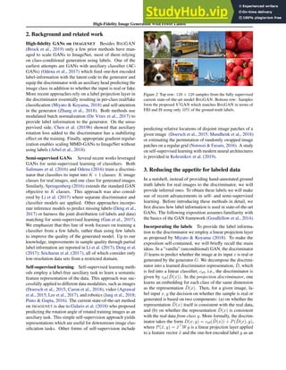
![High-Fidelity Image Generation With Fewer Labels
Mario Lucic * 1
Michael Tschannen * 2
Marvin Ritter * 1
Xiaohua Zhai 1
Olivier Bachem 1
Sylvain Gelly 1
Abstract
Deep generative models are becoming a cor-
nerstone of modern machine learning. Recent
work on conditional generative adversarial net-
works has shown that learning complex, high-
dimensional distributions over natural images is
within reach. While the latest models are able to
generate high-fidelity, diverse natural images at
high resolution, they rely on a vast quantity of
labeled data. In this work we demonstrate how
one can benefit from recent work on self- and
semi-supervised learning to outperform state-of-
the-art (SOTA) on both unsupervised ImageNet
synthesis, as well as in the conditional setting.
In particular, the proposed approach is able to
match the sample quality (as measured by FID) of
the current state-of-the art conditional model Big-
GAN on ImageNet using only 10% of the labels
and outperform it using 20% of the labels.
1. Introduction
Deep generative models have received a great deal of
attention due to their power to learn complex high-
dimensional distributions, such as distributions over nat-
ural images (Zhang et al., 2018; Brock et al., 2019),
videos (Kalchbrenner et al., 2017), and audio (Van Den Oord
et al., 2016). Recent progress was driven by scalable train-
ing of large-scale models (Brock et al., 2019; Menick
Kalchbrenner, 2019), architectural modifications (Zhang
et al., 2018; Chen et al., 2019a; Karras et al., 2018), and
normalization techniques (Miyato et al., 2018).
High-fidelity natural image generation (typically trained
on ImageNet) hinges upon having access to vast quantities
of labeled data. This is unsurprising as labels induce rich
side information into the training process, effectively divid-
ing the extremely challenging image generation task into
semantically meaningful sub-tasks.
*
Equal contribution 1
Google Brain, Zurich, Switzer-
land 2
ETH Zurich, Zurich, Switzerland. Correspondence
to: Mario Lucic lucic@google.com, Michael Tschan-
nen mi.tschannen@gmail.com, Marvin Ritter marvinrit-
ter@google.com.
5 10 15 20 25
FID Score
Random label
Single label
Single label (SS)
Clustering
Clustering (SS)
S2
GAN
S3
GAN
S2
GAN
S3
GAN
S2
GAN
S3
GAN
5% labels
10% labels
20% labels
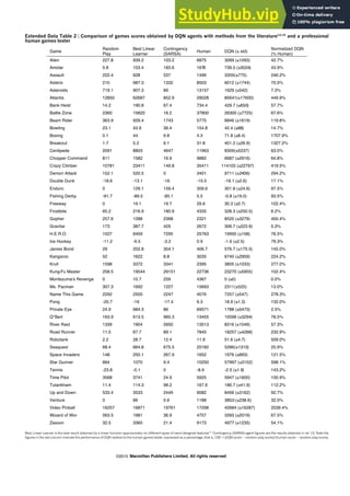
Figure 1. FID of the baselines and the proposed method. The
vertical line indicates the baseline (BigGAN) which uses all the
labeled data. The proposed method (S3
GAN) is able to match
the state-of-the-art while using only 10% of the labeled data and
outperform it with 20%.
However, this dependence on vast quantities of labeled data
is at odds with the fact that most data is unlabeled, and
labeling itself is often costly and error-prone. Despite the
recent progress on unsupervised image generation, the gap
between conditional and unsupervised models in terms of
sample quality is significant.
In this work, we take a significant step towards closing the
gap between conditional and unsupervised generation of
high-fidelity images using generative adversarial networks
(GANs). We leverage two simple yet powerful concepts:
(i) Self-supervised learning: A semantic feature extractor
for the training data can be learned via self-supervision,
and the resulting feature representation can then be
employed to guide the GAN training process.
(ii) Semi-supervised learning: Labels for the entire train-
ing set can be inferred from a small subset of labeled
training images and the inferred labels can be used as
conditional information for GAN training.
Our contributions In this work, we
1. propose and study various approaches to reduce or fully
omit ground-truth label information for natural image
generation tasks,
2. achieve a new SOTA in unsupervised generation on Ima-
geNet, match the SOTA on 128 × 128 IMAGENET using
only 10% of the labels, and set a new SOTA using only
20% of the labels (measured by FID), and
3. open-source all the code used for the experiments at
github.com/google/compare_gan.
arXiv:1903.02271v1
[cs.LG]
6
Mar
2019](https://image.slidesharecdn.com/5importantdeeplearningresearchpapersyoumustreadin2020-230805220002-b1ad183f/85/5-Important-Deep-Learning-Research-Papers-You-Must-Read-In-2020-53-320.jpg)
![High-Fidelity Image Generation With Fewer Labels
D
hat y_R
D
y_F
c
hat y_R
D
D
D
G
yf
z
D̃
xf
xr
yf
cr/f
P
yr
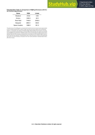
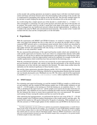
Figure 3. Conditional GAN with projection discriminator. The
discriminator tries to predict from the representation D̃ whether a
real image xr (with label yr) or a generated image xf (with label
yf) is at its input, by combining an unconditional classifier cr/f and
a class-conditional classifier implemented through the projection
layer P. This form of conditioning is used in BIGGAN. Outward-
pointing arrows feed into losses.
input. As for the generator, the label information y is incor-
porated through class-conditional BatchNorm (Dumoulin
et al., 2017; De Vries et al., 2017). The conditional GAN
with projection discriminator is illustrated in Figure 3. We
proceed with describing the pre-trained and co-training ap-
proaches to infer labels for GAN training in Sections 3.1
and 3.2, respectively.
3.1. Pre-trained approaches
Unsupervised clustering-based method We first learn
a representation of the real training data using a state-
of-the-art self-supervised approach (Gidaris et al., 2018;
Kolesnikov et al., 2019), perform clustering on this repre-
sentation, and use the cluster assignments as a replacement
for labels. Following Gidaris et al. (2018) we learn the fea-
ture extractor F (typically a convolutional neural network)
by minimizing the following self-supervision loss
LR = −
1
|R|
X
r∈R
Ex∼pdata(x)[log p(cR(F(xr
)) = r)], (1)
where R is the set of the 4 rotation degrees
{0◦
, 90◦
, 180◦
, 270◦
}, xr
is the image x rotated by
r, and cR is a linear classifier predicting the rotation
degree r. After learning the feature extractor F, we apply
mini batch k-Means clustering (Sculley, 2010) on the
representations of the training images. Finally, given the
cluster assignment function ŷCL = cCL(F(x)) we train the
GAN using the hinge loss, alternatively minimizing the
discriminator loss LD and generator loss LG, namely
LD = −Ex∼pdata(x)[min(0, −1 + D(x, cCL(F(x))))]
− E(z,y)∼p̂(z,y)[min(0, −1 − D(G(z, y), y))]
LG = −E(z,y)∼p̂(z,y)[D(G(z, y), y)],
where p̂(z, y) = p(z)p̂(y) is the prior distribution with
p(z) = N(0, I) and p̂(y) the empirical distribution of the
D
D
G
yf
z
D̃
xf
xr
yf
cr/f
P
F cCL
Figure 4. CLUSTERING: Unsupervised approach based on cluster-
ing the representations obtained by solving a self-supervised task.
F corresponds to the feature extractor learned via self-supervision
and cCL is the cluster assignment function. After learning F and
cCL on the real training images in the pre-training step, we pro-
ceed with conditional GAN training by inferring the labels as
ŷCL = cCL(F(x)).
cluster labels cCL(F(x)) over the training set. We call this
approach CLUSTERING and illustrate it in Figure 4.
Semi-supervised method While semi-supervised learn-
ing is an active area of research and a large variety of al-
gorithms has been proposed, we follow Beyer et al. (2019)
and simply extend the self-supervised approach described
in the previous paragraph with a semi-supervised loss. This
ensures that the two approaches are comparable in terms
of model capacity and computational cost. Assuming we
are provided with labels for a subset of the training data,
we attempt to learn a good feature representation via self-
supervision and simultaneously train a good linear classifier
on the so-obtained representation (using the provided la-
bels).1
More formally, we minimize the loss
LS2
L = −
1
|R|
X
r∈R
n
Ex∼pdata(x)[log p(cR(F(xr
)) = r)]
+ γE(x,y)∼pdata(x,y)[log p(cS2
L(F(xr
)) = y)]
o
,
(2)
where cR and cS2
L are linear classifiers predicting the ro-
tation angle r and the label y, respectively, and γ 0
balances the loss terms. The first term in (2) corresponds to
the self-supervision loss from (1) and the second term to a
(semi-supervised) cross-entropy loss. During training, the
latter expectation is replaced by the empirical average over
the subset of labeled training examples, whereas the former
is set to the empirical average over the entire training set
(this convention is followed throughout the paper). After we
obtain F and cS2
L we proceed with GAN training where we
1
Note that an even simpler approach would be to first learn
the representation via self-supervision and subsequently the linear
classifier, but we observed that learning the representation and
classifier simultaneously leads to better results.](https://image.slidesharecdn.com/5importantdeeplearningresearchpapersyoumustreadin2020-230805220002-b1ad183f/85/5-Important-Deep-Learning-Research-Papers-You-Must-Read-In-2020-55-320.jpg)
![High-Fidelity Image Generation With Fewer Labels
D
G
x_R
x_F
z
y_F
y_F
F c hat y_R
D
y_F
c
hat y_R
D
D
G
yf
z
D̃
xf
xr
yf
cr/f
P
cCT
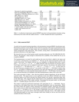
Figure 5. S2
GAN-CO: During GAN training we learn an auxiliary
classifier cCT on the discriminator representation D̃, based on the
labeled real examples, to predict labels for the unlabeled ones.
This avoids training a feature extractor F and classifier cS2
L prior
to GAN training as in S2
GAN.
label the real images as ŷS2
L = cS2
L(F(x)). In particular,
we alternatively minimize the same generator and discrim-
inator losses as for CLUSTERING except that we use cS2
L
and F obtained by minimizing (2):
LD = −Ex∼pdata(x)[min(0, −1 + D(x, cS2
L(F(x))))]
− E(z,y)∼p(z,y)[min(0, −1 − D(G(z, y), y))]
LG = −E(z,y)∼p(z,y)[D(G(z, y), y)],
where p(z, y) = p(z)p(y) with p(z) = N(0, I) and p(y)
uniform categorical. We use the abbreviation S2
GAN for
this method.
3.2. Co-training approach
The main drawback of the transfer-based methods is that
one needs to train a feature extractor F via self supervision
and learn an inference mechanism for the labels (linear clas-
sifier or clustering). In what follows we detail co-training
approaches that avoid this two-step procedure and learn to
infer label information during GAN training.
Unsupervised method We consider two approaches. In
the first one, we completely remove the labels by simply la-
beling all real and generated examples with the same label2
and removing the projection layer from the discriminator,
i.e., we set D(x) = cr/f(D̃(x)). We use the abbreviation
SINGLE LABEL for this method. For the second approach
we assign random labels to (unlabeled) real images. While
the labels for the real images do not provide any useful sig-
nal to the discriminator, the sampled labels could potentially
help the generator by providing additional randomness with
different statistics than z, as well as additional trainable pa-
rameters due to the embedding matrices in class-conditional
BatchNorm. Furthermore, the labels for the fake data could
2
Note that this is not necessarily equivalent to replacing class-
conditional BatchNorm with standard (unconditional) BatchNorm
as the variant of conditional BatchNorm used in this paper also uses
chunks of the latent code as input; besides the label information.
D
G
x_R
x_F
z
y_F
y
F c
D
G
yf
z
D̃
xf
xr
yf
cr/f
P
yr
cR
Figure 6. Self-supervision by rotation-prediction during GAN
training. Additionally to predicting whether the images at its
input are real or generated, the discriminator is trained to predict
rotations of both rotated real and fake images via an auxiliary lin-
ear classifier cR. This approach was successfully applied by Chen
et al. (2019b) to stabilize GAN training. Here we combine it with
our pre-trained and co-training approaches, replacing the ground
truth labels yr with predicted ones.
facilitate the discrimination as they provide side information
about the fake images to the discriminator. We term this
method RANDOM LABEL.
Semi-supervised method When labels are available for a
subset of the real data, we train an auxiliary linear classifier
cCT directly on the feature representation D̃ of the discrimi-
nator, during GAN training, and use it to predict labels for
the unlabeled real images. In this case the discriminator loss
takes the form
LD = − E(x,y)∼pdata(x,y)[min(0, −1 + D(x, y))]
− λE(x,y)∼pdata(x,y)[log p(cCT(D̃(x)) = y)]
− Ex∼pdata(x)[min(0, −1 + D(x, cCT(D̃(x))))]
− E(z,y)∼p(z,y)[min(0, −1 − D(G(z, y), y))], (3)
where the first term corresponds to standard conditional
training on (k%) labeled real images, the second term is
the cross-entropy loss (with weight λ 0) for the auxiliary
classifier cCT on the labeled real images, the third term is
an unsupervised discriminator loss where the labels for the
unlabeled real images are predicted by cCT, and the last
term is the standard conditional discriminator loss on the
generated data. We use the abbreviation S2
GAN-CO for
this method. See Figure 5 for an illustration.
3.3. Self-supervision during GAN training
So far we leveraged self-supervision to either craft good fea-
ture representations, or to learn a semi-supervised model (cf.
Section 3.1). However, given that the discriminator itself
is just a classifier, one may benefit from augmenting this
classifier with an auxiliary task—namely self-supervision
through rotation prediction. This approach was already ex-
plored in (Chen et al., 2019b), where it was observed to
stabilize GAN training. Here we want to assess its impact](https://image.slidesharecdn.com/5importantdeeplearningresearchpapersyoumustreadin2020-230805220002-b1ad183f/85/5-Important-Deep-Learning-Research-Papers-You-Must-Read-In-2020-56-320.jpg)
![High-Fidelity Image Generation With Fewer Labels
when combined with the methods introduced in Sections 3.1
and 3.2. To this end, similarly to the training of F in (1)
and (2), we train an additional linear classifier cR on the
discriminator feature representation D̃ to predict rotations
r ∈ R of the rotated real images xr
and rotated fake im-
ages G(z, y)r
. The corresponding loss terms added to the
discriminator and generator losses are
−
β
|R|
X
r∈R
Ex∼pdata(x)[log p(cR(D̃(xr
) = r)] (4)
and
−
α
|R|
E(z,y)∼p(z,y)[log p(cR(D̃(G(z, y)r
) = r)], (5)
respectively, where α, β 0 are weights to balance the loss
terms. This approach is illustrated in Figure 6.
4. Experimental setup
Architecture and hyperparameters GANs are notori-
ously unstable to train and their performance strongly de-
pends on the capacity of the neural architecture, optimiza-
tion hyperparameters, and appropriate regularization (Lucic
et al., 2018; Kurach et al., 2018). We implemented the con-
ditional BigGAN architecture (Brock et al., 2019) which
achieves state-of-the-art results on ImageNet.3
We use ex-
actly the same optimization hyper-parameters as Brock et al.
(2019). Specifically, we employ the Adam Optimizer with
the learning rates 5 · 10−5
for the generator and 2 · 10−4
for the discriminator (β1 = 0 β2 = 0.999). We train for
250k generator steps with 2 discriminator iterations before
each generator step. The batch size was fixed to 2048, and
we use a latent code z with 120 dimensions. We employ
spectral normalization in both generator and discriminator.
In contrast to BigGAN, we do not apply orthogonal regu-
larization as this was observed to only marginally improve
sample quality (cf. Table 1 in Brock et al. (2019)) and we
do not use the truncation trick.
Datasets We focus primarily on IMAGENET, the largest
and most diverse image data set commonly used to evaluate
GANs. IMAGENET contains 1.3M training images and 50k
test images, each corresponding to one of 1k object classes.
We resize the images to 128 × 128 × 3 as done in Miyato
Koyama (2018) and Zhang et al. (2018). Partially labeled
data sets for the semi-supervised approaches are obtained
by randomly selecting k% of the samples from each class.
3
We dissected the model checkpoints released by Brock et al.
(2019) to obtain exact counts of trainable parameters and their
dimensions, and match them to byte level (cf. Tables 10 and
11). We want to emphasize that at this point this methodology
is bleeding-edge and successful state-of-the-art methods require
careful architecture-level tuning. To foster reproducibility we
meticulously detail this architecture at tensor-level detail in Ap-
pendix B and open-source our code at https://github.com/
google/compare_gan.
Evaluation metrics We use the Fréchet Inception Dis-
tance (FID) (Heusel et al., 2017) and Inception Score (Sal-
imans et al., 2016) to evaluate the quality of the gener-
ated samples. To compute the FID, the real data and
generated samples are first embedded in a specific layer
of a pre-trained Inception network. Then, a multivariate
Gaussian is fit to the data and the distance computed as
FID(x, g) = ||µx − µg||2
2 + Tr(Σx + Σg − 2(ΣxΣg)
1
2 ),
where µ and Σ denote the empirical mean and covariance,
and subscripts x and g denote the real and generated data
respectively. FID was shown to be sensitive to both the addi-
tion of spurious modes and to mode dropping (Sajjadi et al.,
2018; Lucic et al., 2018). Inception Score posits that condi-
tional label distribution of samples containing meaningful
objects should have low entropy, and the variability of the
samples should be high leading to the following formula-
tion: IS = exp(Ex∼Q[dKL(p(y | x), p(y))]). Although it
has some flaws (Barratt Sharma, 2018), we report it to en-
able comparison with existing methods. Following (Brock
et al., 2019), the FID is computed using the 50k IMAGENET
testing images and 50k randomly sampled fake images, and
the IS is computed from 50k randomly sampled fake images.
All metrics are computed for 5 different randomly sampled
sets of fake images and we report the mean.
Methods We conduct an extensive comparison of meth-
ods detailed in Table 1, namely: Unmodified BIGGAN, the
unsupervised methods SINGLE LABEL, RANDOM LABEL,
CLUSTERING, and the semi-supervised methods S2
GAN
and S2
GAN-CO. In all S2
GAN-CO experiments we use
soft labels, i.e., the soft-max output of cCT instead of one-
hot encoded hard estimates, as we observed in preliminary
experiments that this stabilizes training. For S2
GAN we use
hard labels by default, but investigate the effect of soft labels
in separate experiments. For all semi-supervised methods
we have access only to k% of the ground truth labels where
k ∈ {5, 10, 20}. As an additional baseline, we retain k%
labeled real images and discard all unlabeled real images,
then using the remaining labeled images to train BIGGAN
(the resulting model is designated by BIGGAN-k%). Fi-
nally, we explore the effect of self-supervision during GAN
training on the unsupervised and semi-supervised methods.
We train every model three times with a different random
seed and report the median FID and the median IS. With
the exception of the SINGLE LABEL and BIGGAN-k%, the
standard deviation of the mean across three runs is very
low. We therefore defer tables with the mean FID and IS
values and standard deviations to Appendix D. All models
are trained on 128 cores of a Google TPU v3 Pod with
BatchNorm statistics synchronized across cores.
Unsupervised approaches For CLUSTERING we sim-
ply used the best available self-supervised rotation
model from (Kolesnikov et al., 2019). The number](https://image.slidesharecdn.com/5importantdeeplearningresearchpapersyoumustreadin2020-230805220002-b1ad183f/85/5-Important-Deep-Learning-Research-Papers-You-Must-Read-In-2020-57-320.jpg)

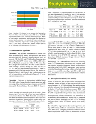
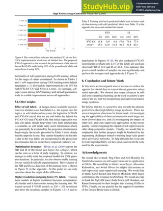
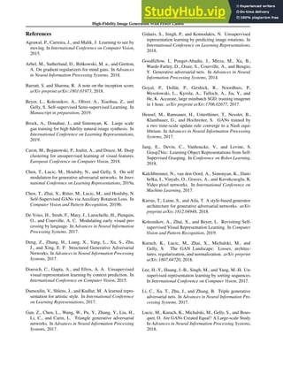
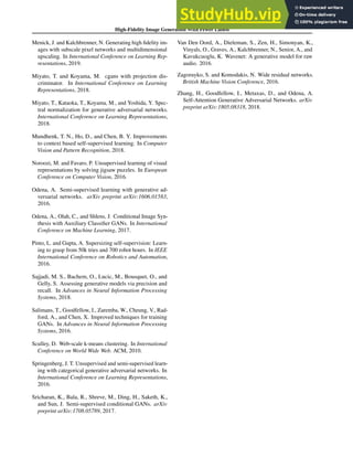
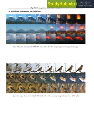
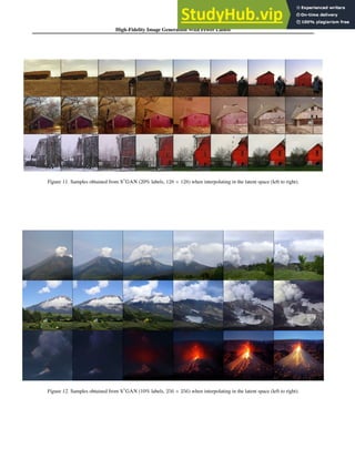
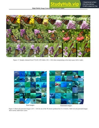
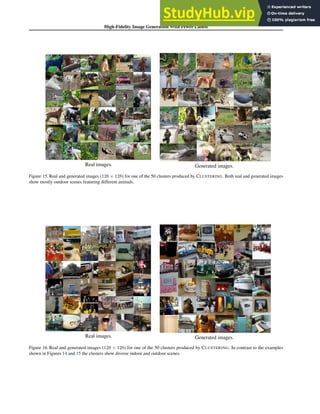
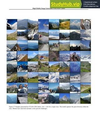
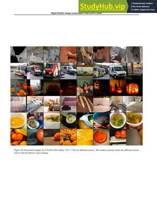
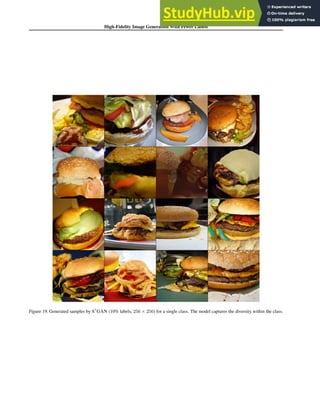
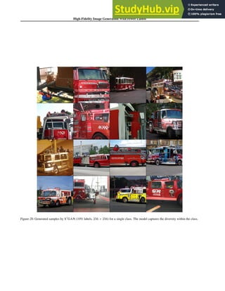
![High-Fidelity Image Generation With Fewer Labels
B. Architectural details
The ResNet architecture implemented following Brock
et al. (2019) is described in Tables 6 and 7. We use
the abbreviations RS for resample and BN for batch
normalization. In the resample column, we indicate
downscale(D)/upscale(U)/none(-) setting. In Table 7, y
stands for the labels and h is the output from the layer be-
fore (i.e., the pre-logit layer). Tables 8 and 9 show ResBlock
details. The addition layer merges the shortcut path and the
convolution path by adding them. h and w are the input
height and width of the ResBlock, ci and co are the input
channels and output channels for a ResBlock. For the last
ResBlock in the discriminator without resampling, we sim-
ply drop the shortcut layer from ResBlock. We list all the
trainable variables and their shape in Tables 10 and 11.
Table 6. ResNet generator architecture. “ch” represents the channel
width multiplier and is set to 96.
LAYER RS OUTPUT
z ∼ N(0, 1) - 120
Dense - 4 × 4 × 16 · ch
ResBlock U 8 × 8 × 16 · ch
ResBlock U 16 × 16 × 8 · ch
ResBlock U 32 × 32 × 4 · ch
ResBlock U 64 × 64 × 2 · ch
Non-local block - 64 × 64 × 2 · ch
ResBlock U 128 × 128 × 1 · ch
BN, ReLU - 128 × 128 × 3
Conv [3, 3, 1] - 128 × 128 × 3
Tanh - 128 × 128 × 3
Table 7. ResNet discriminator architecture. “ch” represents the
channel width multiplier and is set to 96.
LAYER RS OUTPUT
Input image - 128 × 128 × 3
ResBlock D 64 × 64 × 1 · ch
Non-local block - 64 × 64 × 1 · ch
ResBlock D 32 × 32 × 2 · ch
ResBlock D 16 × 16 × 4 · ch
ResBlock D 8 × 8 × 8 · ch
ResBlock D 4 × 4 × 16 · ch
ResBlock - 4 × 4 × 16 · ch
ReLU - 4 × 4 × 16 · ch
Global sum pooling - 1 × 1 × 16 · ch
Sum(embed(y)·h)+(dense→ 1) - 1
Table 8. ResBlock discriminator.
LAYER KERNEL RS OUTPUT
Shortcut [1, 1, 1] D h/2 × w/2 × co
BN, ReLU - - h × w × ci
Conv [3, 3, 1] - h × w × co
BN, ReLU - - h × w × co
Conv [3, 3, 1] D h/2 × w/2 × co
Addition - - h/2 × w/2 × co
Table 9. ResBlock generator.
LAYER KERNEL RS OUTPUT
Shortcut [1, 1, 1] U 2h × 2w × co
BN, ReLU - - h × w × ci
Conv [3, 3, 1] U 2h × 2w × co
BN, ReLU - - 2h × 2w × co
Conv [3, 3, 1] - 2h × 2w × co
Addition - - 2h × 2w × co](https://image.slidesharecdn.com/5importantdeeplearningresearchpapersyoumustreadin2020-230805220002-b1ad183f/85/5-Important-Deep-Learning-Research-Papers-You-Must-Read-In-2020-71-320.jpg)
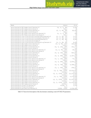
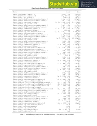
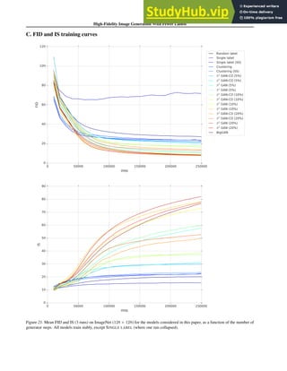
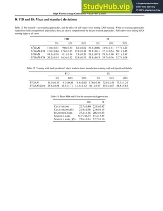

The document summarizes 5 important deep learning research papers from 2020. It discusses a paper on using deep reinforcement learning to achieve human-level control. It also mentions papers on deep learning applications for clothing image analysis, semi-supervised learning, graph representation learning with PyTorch, and high-fidelity image generation with fewer labels.