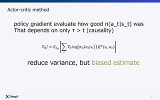
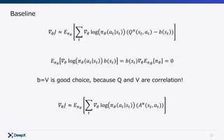
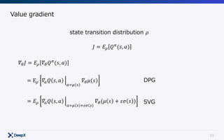
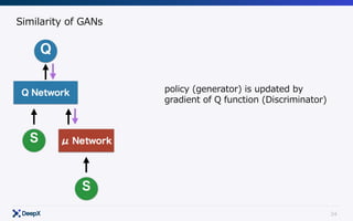
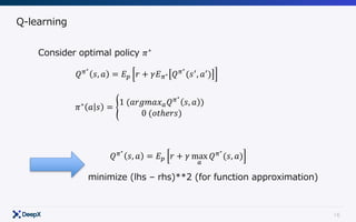
This document discusses model-free continuous control in reinforcement learning. It introduces policy gradient and value gradient methods for learning continuous control policies with neural networks. Policy gradient methods directly optimize the policy parameters with the policy gradient. Value gradient methods optimize the policy based on the gradient of a learned state-action value function. Actor-critic methods combine policy gradients with value functions to reduce variance.

![8
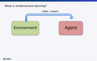
Formulation
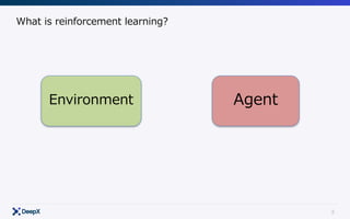
Agent
Environment
𝐴"~𝜋(𝑎|𝑆")
𝑆"*+~𝑃(𝑠.
|𝑆", 𝐴")
𝑟"*+ = 𝑟(𝑆", 𝐴", 𝑆"*+)
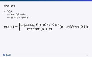
Modeling π!
π∗
= argmax
π
Eπ [ γ τ
rτ ]
τ =0
∞
∑Get
Model-free](https://image.slidesharecdn.com/continuouscontrol-170822073400/85/Continuous-control-8-320.jpg)
![9
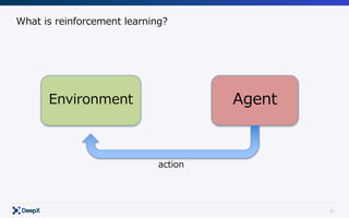
Formulation
Agent
Environment
𝐴"~𝜋(𝑎|𝑆")
𝑆"*+~𝑃(𝑠.
|𝑆", 𝐴")
𝑟"*+ = 𝑟(𝑆", 𝐴", 𝑆"*+)
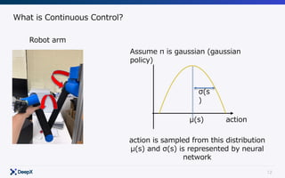
Modeling π and P!
π∗
= argmax
π
Eπ [ γ τ
rτ ]
τ =0
∞
∑Get
Model-base](https://image.slidesharecdn.com/continuouscontrol-170822073400/85/Continuous-control-9-320.jpg)


![20
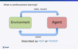
Formulation
Agent
Environment
𝐴"~𝜋(𝑎|𝑆")
𝑆"*+~𝑃(𝑠.
|𝑆", 𝐴")
𝑟"*+ = 𝑟(𝑆", 𝐴", 𝑆"*+)
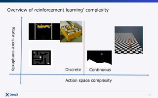
Modeling π!
π∗
= argmax
π
Eπ [ γ τ
rτ ]
τ =0
∞
∑Get
Model-free](https://image.slidesharecdn.com/continuouscontrol-170822073400/85/Continuous-control-20-320.jpg)
![22
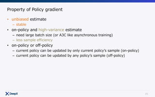
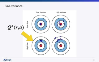
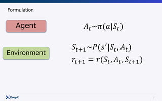
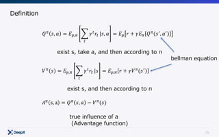
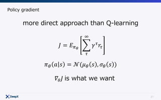
Policy gradient
∇θ J = ∇θ Eπθ
[ γ τ
rτ ]
τ =0
∞
∑
= ∇θ Es0 ~ρ,s'~p πθ at ,st( ) γ τ
rτ
τ =0
∞
∑t=0
∏
⎡
⎣
⎢
⎤
⎦
⎥
= Es0 ~ρ,s'~p ∇θ πθ at ,st( ) γ τ
rτ
τ =0
∞
∑t=0
∏
⎡
⎣
⎢
⎤
⎦
⎥
= Es~ρ πθ at ,st( )
∇θ πθ at ,st( )
t=0
∏
πθ at ,st( )
t=0
∏
γ τ
rτ
τ =0
∞
∑
t=0
∏
⎡
⎣
⎢
⎢
⎢
⎤
⎦
⎥
⎥
⎥
= Es~ρ πθ (at | st ) ∇θ log(πθ (at | st ))
t=0
∑t=0
∏ γ τ
rτ
τ =0
∞
∑
⎡
⎣
⎢
⎤
⎦
⎥
= Eπθ
[ ∇θ log(πθ (at | st ))
t=0
∑ γ τ
rτ
τ =t
∞
∑ ]
Expectation to summation
differentiate w.r.t theta
multiple pi to
nominator and denominator
logarithmic differentiation
Causality
Approximated by MC](https://image.slidesharecdn.com/continuouscontrol-170822073400/85/Continuous-control-22-320.jpg)