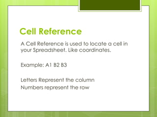
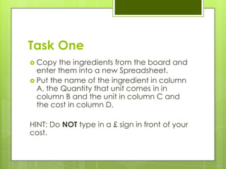
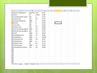
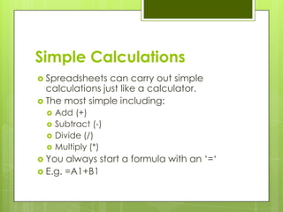
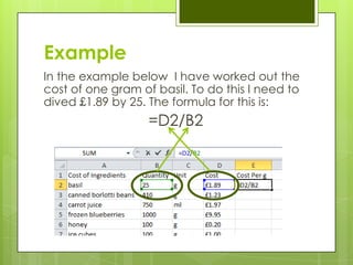
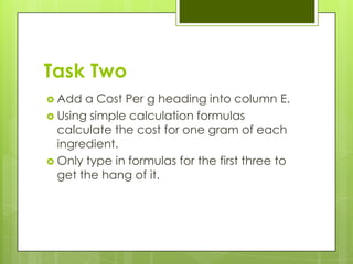
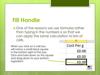
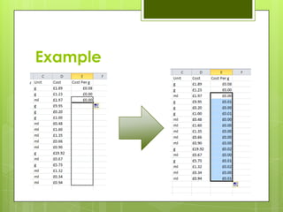
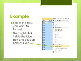
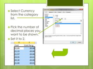
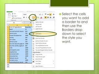
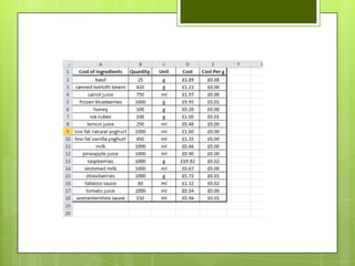
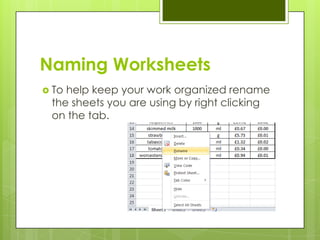
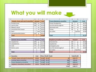
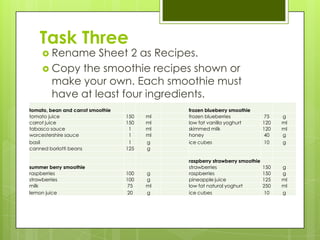
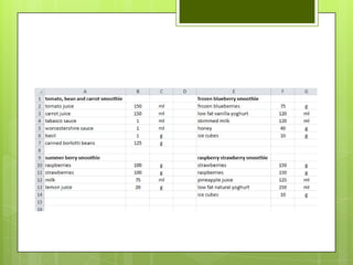
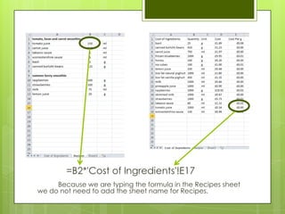
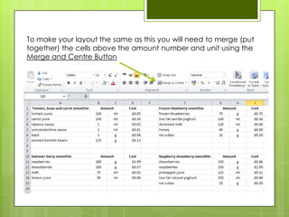
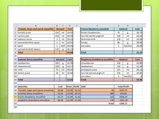
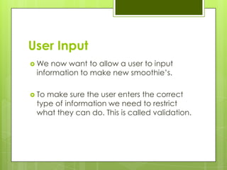
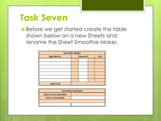
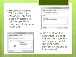
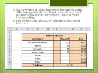
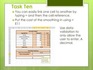
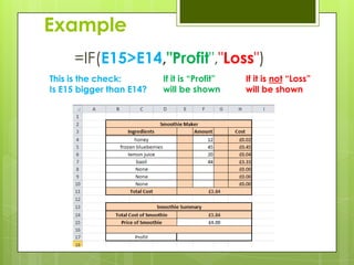
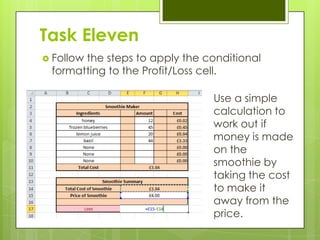
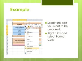
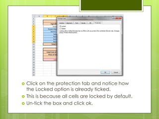
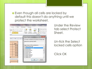
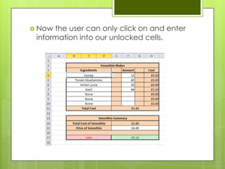
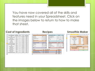
Spreadsheets
Skills Builder
Creating A Simple Spreadsheet –
      What you will make
Cell Reference
A Cell Reference is used to locate a cell in
your Spreadsheet. Like coordinates.

Example: A1 B2 B3

Letters Represent the column
Numbers represent the row
Entering Data
 To
   enter data simply click in the cell you
 want to enter data into and type.
Task One
 Copy  the ingredients from the board and
  enter them into a new Spreadsheet.
 Put the name of the ingredient in column
  A, the Quantity that unit comes in in
  column B and the unit in column C and
  the cost in column D.

HINT: Do NOT type in a £ sign in front of your
cost.
Simple Calculations
 Spreadsheets   can carry out simple
  calculations just like a calculator.
 The most simple including:
     Add (+)
     Subtract (-)
     Divide (/)
     Multiply (*)
 You  always start a formula with an „=„
 E.g. =A1+B1
Example
In the example below I have worked out the
cost of one gram of basil. To do this I need to
dived £1.89 by 25. The formula for this is:
                   =D2/B2
Task Two
 Add  a Cost Per g heading into column E.
 Using simple calculation formulas
  calculate the cost for one gram of each
  ingredient.
 Only type in formulas for the first three to
  get the hang of it.
Fill Handle
  One     of the reasons we use formulas rather
    than typing in the numbers is so that we
    can apply the same calculation to lots of
    cells.
When you click on a cell you
will notice a small black square
in the bottom right of the box.
Click and hold down on this square
and drag down to your bottom
ingredient.
Example
Relative Cell Reference
 You  should now notice that the same
 calculation has been copied down and
 all the letters in the formula have stayed
 the same but the numbers have changed
 to the number for the row they are in.

    This is what is called a relative cell
                 reference.
Cell Formatting
 Your   might have automatically formatted
  your cost to currency and put a £ in front
  of your numbers.
 If not you will need to format the cells.
 Formatting is your way of telling the
  Spreadsheet what type of data is in the
  cell. i.e. Currency, Number, Text
Example
 Select  the cells
  you want to
  format.
 Then right click
  inside the blue
  box and click on
  Format Cells.
 SelectCurrency
 from the category
 list.

 Pick  the number of
  decimal places you
  want to be shown.
 Set it to 2.
Making it look good
 Now  we have finished our simple
  Spreadsheet we need to make it look
  neater.
 Using Boarders and Aligning text we can
  make a table look clearer and more
  professional.
 Select the cells
           you want to add
Example    a border to and
           then use the
           Borders drop
           down to select
           the style you
           want.
Naming Worksheets
 Tohelp keep your work organized rename
 the sheets you are using by right clicking
 on the tab.
Formulas and Functions
 Weare now going to create a more
 complex Spreadsheet using functions.

A   function is a pre programed calculation
  in the software that you only need to
  enter the name of to make it perform the
  calculation.
 E.g. SUM, MIN, MAX
What you will make
Task Three
      Rename   Sheet 2 as Recipes.
      Copy the smoothie recipes shown or
       make your own. Each smoothie must
       have at least four ingredients.
tomato, bean and carrot smoothie              frozen blueberry smoothie
tomato juice                       150   ml   frozen blueberries               75   g
carrot juice                       150   ml   low fat vanilla yoghurt         120   ml
tabasco sauce                       1    ml   skimmed milk                    120   ml
worcestershire sauce                1    ml   honey                            40   g
basil                               1    g    ice cubes                        10   g
canned borlotti beans              125   g

                                              raspberry strawberry smoothie
summer berry smoothie                         strawberries                    150   g
raspberries                        100   g    raspberries                     150   g
strawberries                       100   g    pineapple juice                 125   ml
milk                                75   ml   low fat natural yoghurt         250   ml
lemon juice                         20   g    ice cubes                        10   g
Linking Sheets Together
 Notonly can you use formulas to do
 calculations with data on a sheet but you
 can also do it with information on different
 sheets.

 Todo this we need to add the name of
 the sheet in front of the cell reference.
Example
 Towork of the cost of the ingredients used
 in each smoothie we need to multiply the
 amount used in the smoothie which is on
 the Recipes sheet by the cost of a single g
 of the ingredient which is on the Cost of
 Ingredients sheet.


Hint: Excel will do this automatically when
you click in the cell you are using.
=B2*'Cost of Ingredients'!E17
     Because we are typing the formula in the Recipes sheet
we do not need to add the sheet name for Recipes.
Task Four
 Usea simple formula to calculate the cost
 of each ingredient in the smoothie by
 multiplying the amount use by the cost for
 a gram.

Note: Using the auto fill handle wont work
here! Why not?
To make your layout the same as this you will need to merge (put
together) the cells above the amount number and unit using the
Merge and Centre Button
SUM Function
 TheSUM function will add a list of numbers
 together. This is useful as it is easier than
 using individual cell references.

E.g.
   = A1 + A2 + A3 +A4 + A5 + A6 + A7 + A8
                     vs.
                = SUM(A1:A8)
Task Five
 Usethe SUM function to add all of the
 ingredients for each smoothie together.

 Youhave four smoothie‟s so you will need
 to write 4 SUM functions.
Example
Borders and Shading
 Just
     as we added boarders before now
 add borders and shading to make the
 tables look better.
Task Six
   Now we you know how to use formulas and
    functions make a summary table that will show
    much profit would be made if the numbers shown
    below for £2.80 each.

   It should look like this.
User Input
 We now want to allow a user to input
 information to make new smoothie‟s.

 Tomake sure the user enters the correct
 type of information we need to restrict
 what they can do. This is called validation.
What you will make
Task Seven
 Before
       we get started create the table
 shown below on a new Sheets and
 rename the Sheet Smoothie Maker.
Dropdown Boxes
 One    great way of controlling a users input
  is using drop boxes.

 Thisis what we will use to allow the user to
  enter the ingredients they want to use in
  the new smoothie.
Example


 Select   the cells you want to be drop
  boxes
 Select the Data Tab and click on data
  validation.
   Select list from the
    allow menu.
   Click on the Source
    and select the
    ingredients in your
    Spreadsheet.
   Click Ok


Note: I have included a None ingredient
Task Eight
 Follow  the
  steps to add
  dropdown
  boxes.
 When you
  click in these
  Cells a drop
  down box
  should
  appear.
Data Validation
 It
   would be impractical to use a
  dropdown box when entering the amount
  as this could be anything number
  between 1 and 1000.

 Another   way of restricting a user's input is
  to only allow them to enter one type of
  data . i.e. Number, Date, Text
Example
   Again select the cells you want to
    validate. Click the Data Tab and click on
    data validation.

 Thistime pick Whole
  Number from the list
  and enter a
  Minimum number
  and a Maximum.
 Before  clicking ok.
 Click on the Input
 Message Tab and
 add a message to
 tell the user what
 they need to type in
 these cells.

                          Then click on the
                          Error Alert Tab and
                          add a message that
                          will appear should
                          the user enter
                          something incorrect
                          into the cell.
Vlookup
   Now that the user can enter a ingredient from
    a list and type the amount of that ingredient
    they want we need to calculate the cost.
   Because the ingredient entered will not
    always be the same we cant use a normal
    cell reference to the ingredients cost.
   What we need to do is LOOKUP the cost using
    the name of the ingredient
Example
                                            ,
   =VLOOKUP(B4,'Cost of Ingredients'!A2:E19 5)
                   The table you       The number
The name you                           of the column
                   are looking for
are looking up                         you want returned
                   The name in
                                       in that table


                                        1       2 3 4   5
=VLOOKUP(B4,'Cost of Ingredients'!A2:E19,5)*Sheet1!F4

Now you have looked up the cost for that ingredient you
need to multiply it by the amount.

Try: What happens if you try and use the auto fill. Does it
work? Why does it not work? If it looks like it works try
changing one of your ingredients to basil.


                                              Why is this not
                                              working?
Absolute Cell Referencing
   The reason it doesn‟t
    work is because we
    have used relative cell
    references so as we
    dragged the auto fill
    down the position of
    where we were looking
    for our table moved.
   As you can see the
    table has moved
    down and can no
    longer see some of the
    ingredients.
Absolute Cell Referencing
 What    we need to do is lock some of the cell
  references so that they don‟t change when using
  auto fill.
 This is what absolute cell referencing is.
 Its really simple to do too. Just add a $ in front of
  the letter and number you want to lock.

 =VLOOKUP(B4,'Cost of Ingredients'!$A$2:$E$18,5)

  These cells are not locked and these are locked
Hint: If you select a cell reference and press F4 it
will lock it
   We now have a table that allows the user to select
    different ingredients and there amounts and it will
    automatically tell you how much it cost to make
    that smoothie.
   You will need to use a SUM function to add up all
    the costs.
Task Ten
 You  can easily link one cell to another by
  typing = and then the cell reference.
 Put the cost of the smoothing in using =
  E11
                                   Use data
                                   validation to
                                   only allow the
                                   user to enter. A
                                   decimal.
IF Function
 An if function will return an answer IF
  something is true.

 We   will use this to Return the Word “Profit”
  if the smoothie made is cheaper to make
  than the Price entered by the user.
 It will return “Loss” if it is more expensive.
Example
     =IF(E15>E14,"Profit","Loss")
This is the check:        If it is “Profit”   If it is not “Loss”
Is E15 bigger than E14?   will be shown       will be shown
Conditional Formatting
 Conditionalformatting allows us to
  change the colour and shading of cells
  depending on what data is in them.

 This   is useful to highlight information.
Example
To apply conditional formatting select the
cell you want to format and click on
conditional formatting. We are going to use
the highlight cells rule use text that contains.
 Type    Profit into the box and select green
  fill from the list.
 Then apply formatting again to the same
  cell but enter Loss into the box and Red Fill
Now if a Profit is
made it will appear
light Green.


                      Now if a Loss is
                      made it will appear
                      light Red.
Task Eleven
 Follow
       the steps to apply the conditional
 formatting to the Profit/Loss cell.

                               Use a simple
                               calculation to
                               work out if
                               money is made
                               on the
                               smoothie by
                               taking the cost
                               to make it
                               away from the
                               price.
Task Twelve
   Apply conditional
    formatting to
    highlight the cell
    green if the
    number is greater
    than 0 and red if
    it is less than 0.01.
Protecting Cells
 To stop the user from changing the titles
  and any formulas used we need to lock
  those cells.
 The only cells we want unlocked are the
  ones where the users needs to input
  information.
Example

           Select the cells
            you want to be
            unlocked.
           Right click and
            select Format
            Cells.
   Click on the protection tab and notice how
    the Locked option is already ticked.
   This is because all cells are locked by default.
   Un-tick the box and click ok.
 Eventhough all cells are locked by
 default this doesn't do anything until we
 protect the worksheet.
                            Under the Review
                            tab select Protect
                            Sheet.

                            Un-tick the Select
                            locked cells option

                            Click OK
 Now the user can only click on and enter
 information into our unlocked cells.
You have now covered all of the skills and
     features need in your Spreadsheet. Click on
     the images below to return to how to make
     that sheet.

Cost of Ingredients     Recipes         Smoothie Maker

Spreadsheets

  • 1.
  • 2.
    Creating A SimpleSpreadsheet – What you will make
  • 3.
    Cell Reference A CellReference is used to locate a cell in your Spreadsheet. Like coordinates. Example: A1 B2 B3 Letters Represent the column Numbers represent the row
  • 4.
    Entering Data  To enter data simply click in the cell you want to enter data into and type.
  • 5.
    Task One  Copy the ingredients from the board and enter them into a new Spreadsheet.  Put the name of the ingredient in column A, the Quantity that unit comes in in column B and the unit in column C and the cost in column D. HINT: Do NOT type in a £ sign in front of your cost.
  • 7.
    Simple Calculations  Spreadsheets can carry out simple calculations just like a calculator.  The most simple including:  Add (+)  Subtract (-)  Divide (/)  Multiply (*)  You always start a formula with an „=„  E.g. =A1+B1
  • 8.
    Example In the examplebelow I have worked out the cost of one gram of basil. To do this I need to dived £1.89 by 25. The formula for this is: =D2/B2
  • 9.
    Task Two  Add a Cost Per g heading into column E.  Using simple calculation formulas calculate the cost for one gram of each ingredient.  Only type in formulas for the first three to get the hang of it.
  • 10.
    Fill Handle One of the reasons we use formulas rather than typing in the numbers is so that we can apply the same calculation to lots of cells. When you click on a cell you will notice a small black square in the bottom right of the box. Click and hold down on this square and drag down to your bottom ingredient.
  • 11.
  • 12.
    Relative Cell Reference You should now notice that the same calculation has been copied down and all the letters in the formula have stayed the same but the numbers have changed to the number for the row they are in. This is what is called a relative cell reference.
  • 13.
    Cell Formatting  Your might have automatically formatted your cost to currency and put a £ in front of your numbers.  If not you will need to format the cells.  Formatting is your way of telling the Spreadsheet what type of data is in the cell. i.e. Currency, Number, Text
  • 14.
    Example  Select the cells you want to format.  Then right click inside the blue box and click on Format Cells.
  • 15.
     SelectCurrency fromthe category list.  Pick the number of decimal places you want to be shown.  Set it to 2.
  • 16.
    Making it lookgood  Now we have finished our simple Spreadsheet we need to make it look neater.  Using Boarders and Aligning text we can make a table look clearer and more professional.
  • 17.
     Select thecells you want to add Example a border to and then use the Borders drop down to select the style you want.
  • 19.
    Naming Worksheets  Tohelpkeep your work organized rename the sheets you are using by right clicking on the tab.
  • 20.
    Formulas and Functions Weare now going to create a more complex Spreadsheet using functions. A function is a pre programed calculation in the software that you only need to enter the name of to make it perform the calculation.  E.g. SUM, MIN, MAX
  • 21.
  • 22.
    Task Three  Rename Sheet 2 as Recipes.  Copy the smoothie recipes shown or make your own. Each smoothie must have at least four ingredients. tomato, bean and carrot smoothie frozen blueberry smoothie tomato juice 150 ml frozen blueberries 75 g carrot juice 150 ml low fat vanilla yoghurt 120 ml tabasco sauce 1 ml skimmed milk 120 ml worcestershire sauce 1 ml honey 40 g basil 1 g ice cubes 10 g canned borlotti beans 125 g raspberry strawberry smoothie summer berry smoothie strawberries 150 g raspberries 100 g raspberries 150 g strawberries 100 g pineapple juice 125 ml milk 75 ml low fat natural yoghurt 250 ml lemon juice 20 g ice cubes 10 g
  • 24.
    Linking Sheets Together Notonly can you use formulas to do calculations with data on a sheet but you can also do it with information on different sheets.  Todo this we need to add the name of the sheet in front of the cell reference.
  • 25.
    Example  Towork ofthe cost of the ingredients used in each smoothie we need to multiply the amount used in the smoothie which is on the Recipes sheet by the cost of a single g of the ingredient which is on the Cost of Ingredients sheet. Hint: Excel will do this automatically when you click in the cell you are using.
  • 26.
    =B2*'Cost of Ingredients'!E17 Because we are typing the formula in the Recipes sheet we do not need to add the sheet name for Recipes.
  • 27.
    Task Four  Useasimple formula to calculate the cost of each ingredient in the smoothie by multiplying the amount use by the cost for a gram. Note: Using the auto fill handle wont work here! Why not?
  • 28.
    To make yourlayout the same as this you will need to merge (put together) the cells above the amount number and unit using the Merge and Centre Button
  • 29.
    SUM Function  TheSUMfunction will add a list of numbers together. This is useful as it is easier than using individual cell references. E.g. = A1 + A2 + A3 +A4 + A5 + A6 + A7 + A8 vs. = SUM(A1:A8)
  • 30.
    Task Five  UsetheSUM function to add all of the ingredients for each smoothie together.  Youhave four smoothie‟s so you will need to write 4 SUM functions.
  • 31.
  • 32.
    Borders and Shading Just as we added boarders before now add borders and shading to make the tables look better.
  • 34.
    Task Six  Now we you know how to use formulas and functions make a summary table that will show much profit would be made if the numbers shown below for £2.80 each.  It should look like this.
  • 36.
    User Input  Wenow want to allow a user to input information to make new smoothie‟s.  Tomake sure the user enters the correct type of information we need to restrict what they can do. This is called validation.
  • 37.
  • 38.
    Task Seven  Before we get started create the table shown below on a new Sheets and rename the Sheet Smoothie Maker.
  • 39.
    Dropdown Boxes  One great way of controlling a users input is using drop boxes.  Thisis what we will use to allow the user to enter the ingredients they want to use in the new smoothie.
  • 40.
    Example  Select the cells you want to be drop boxes  Select the Data Tab and click on data validation.
  • 41.
    Select list from the allow menu.  Click on the Source and select the ingredients in your Spreadsheet.  Click Ok Note: I have included a None ingredient
  • 42.
    Task Eight  Follow the steps to add dropdown boxes.  When you click in these Cells a drop down box should appear.
  • 43.
    Data Validation  It would be impractical to use a dropdown box when entering the amount as this could be anything number between 1 and 1000.  Another way of restricting a user's input is to only allow them to enter one type of data . i.e. Number, Date, Text
  • 44.
    Example Again select the cells you want to validate. Click the Data Tab and click on data validation.  Thistime pick Whole Number from the list and enter a Minimum number and a Maximum.
  • 45.
     Before clicking ok. Click on the Input Message Tab and add a message to tell the user what they need to type in these cells.  Then click on the Error Alert Tab and add a message that will appear should the user enter something incorrect into the cell.
  • 46.
    Vlookup  Now that the user can enter a ingredient from a list and type the amount of that ingredient they want we need to calculate the cost.  Because the ingredient entered will not always be the same we cant use a normal cell reference to the ingredients cost.  What we need to do is LOOKUP the cost using the name of the ingredient
  • 47.
    Example , =VLOOKUP(B4,'Cost of Ingredients'!A2:E19 5) The table you The number The name you of the column are looking for are looking up you want returned The name in in that table 1 2 3 4 5
  • 48.
    =VLOOKUP(B4,'Cost of Ingredients'!A2:E19,5)*Sheet1!F4 Nowyou have looked up the cost for that ingredient you need to multiply it by the amount. Try: What happens if you try and use the auto fill. Does it work? Why does it not work? If it looks like it works try changing one of your ingredients to basil. Why is this not working?
  • 49.
    Absolute Cell Referencing  The reason it doesn‟t work is because we have used relative cell references so as we dragged the auto fill down the position of where we were looking for our table moved.  As you can see the table has moved down and can no longer see some of the ingredients.
  • 50.
    Absolute Cell Referencing What we need to do is lock some of the cell references so that they don‟t change when using auto fill.  This is what absolute cell referencing is.  Its really simple to do too. Just add a $ in front of the letter and number you want to lock. =VLOOKUP(B4,'Cost of Ingredients'!$A$2:$E$18,5) These cells are not locked and these are locked Hint: If you select a cell reference and press F4 it will lock it
  • 51.
    We now have a table that allows the user to select different ingredients and there amounts and it will automatically tell you how much it cost to make that smoothie.  You will need to use a SUM function to add up all the costs.
  • 52.
    Task Ten  You can easily link one cell to another by typing = and then the cell reference.  Put the cost of the smoothing in using = E11 Use data validation to only allow the user to enter. A decimal.
  • 53.
    IF Function  Anif function will return an answer IF something is true.  We will use this to Return the Word “Profit” if the smoothie made is cheaper to make than the Price entered by the user.  It will return “Loss” if it is more expensive.
  • 54.
    Example =IF(E15>E14,"Profit","Loss") This is the check: If it is “Profit” If it is not “Loss” Is E15 bigger than E14? will be shown will be shown
  • 55.
    Conditional Formatting  Conditionalformattingallows us to change the colour and shading of cells depending on what data is in them.  This is useful to highlight information.
  • 56.
    Example To apply conditionalformatting select the cell you want to format and click on conditional formatting. We are going to use the highlight cells rule use text that contains.
  • 57.
     Type Profit into the box and select green fill from the list.  Then apply formatting again to the same cell but enter Loss into the box and Red Fill
  • 58.
    Now if aProfit is made it will appear light Green. Now if a Loss is made it will appear light Red.
  • 59.
    Task Eleven  Follow the steps to apply the conditional formatting to the Profit/Loss cell. Use a simple calculation to work out if money is made on the smoothie by taking the cost to make it away from the price.
  • 60.
    Task Twelve  Apply conditional formatting to highlight the cell green if the number is greater than 0 and red if it is less than 0.01.
  • 61.
    Protecting Cells  Tostop the user from changing the titles and any formulas used we need to lock those cells.  The only cells we want unlocked are the ones where the users needs to input information.
  • 62.
    Example  Select the cells you want to be unlocked.  Right click and select Format Cells.
  • 63.
    Click on the protection tab and notice how the Locked option is already ticked.  This is because all cells are locked by default.  Un-tick the box and click ok.
  • 64.
     Eventhough allcells are locked by default this doesn't do anything until we protect the worksheet. Under the Review tab select Protect Sheet. Un-tick the Select locked cells option Click OK
  • 65.
     Now theuser can only click on and enter information into our unlocked cells.
  • 66.
    You have nowcovered all of the skills and features need in your Spreadsheet. Click on the images below to return to how to make that sheet. Cost of Ingredients Recipes Smoothie Maker