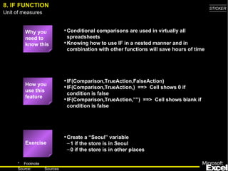
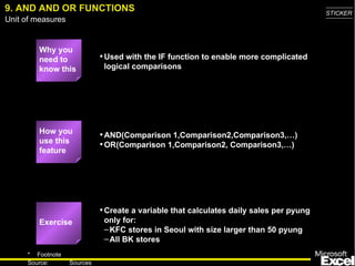
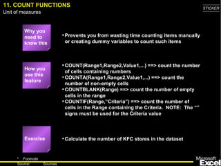
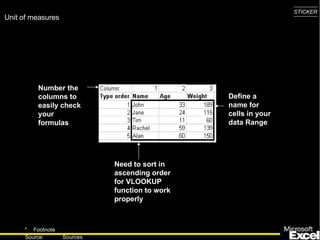
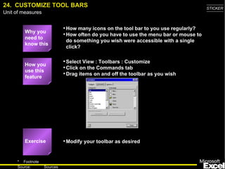
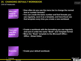
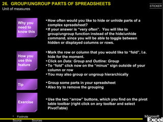
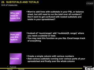
31 Excel Tips   That Could Save You from Working All Night - Version 1.2 -   Cuong Do, Berthold Trenkel-Bögle October 19, 2000
INTRODUCTORY NOTE What is it:  The following material was developed for the Seoul office training program.  Target audience:  1st year associates and business analysts, although there is nothing wrong doing this training as well with EMs and APs.  Duration:  3-4 hours to walk through the explanations and give everyone a chance to actually practice. Faculty:  SEO did it with 2 MGMs, which was extremely powerful, since the seniors showed that they can do and therefore they can expect their team members to do the same. Final comment:  The original material was not intended for self-study purposes and therefore may be a little be too brief and cryptic in some cases. In case you have any improvement ideas please feel free to e-mail them to the authors.
31 EXCEL TIPS THAT COULD SAVE YOU FROM  WORKING ALL NIGHT 1. Split windows and freeze panes 2. Hide  and  Unhide  command 3. Moving around a spreadsheet with Ctrl, Shift, and Arrow keys 4. Name  cells/ranges 5. Sort  command 6. Toggling among relational and absolute references 7. Fill down  and  fill right  commands 8. IF  function 9. AND  and  OR  functions 10. SUM  and  SUMIF  functions 11. COUNT  functions 12. ROUND, ROUNDUP  and  ROUNDDOWN  functions 13. VLOOKUP  and  HLOOKUP  functions 14. Insert Function  command 15. Paste Special  command 16. Auditing features 17. Goal Seek  add-in 18. Solver  add-in 19. Data tables 20. Scenarios  add-in 21. Pivot Tables 22. Protecting cells and worksheets 23. Editing multiple worksheets simultaneously 24. Customize tool bars 25. Changing default workbook 26. Group  and  Ungroup  your spreadsheet 27. Switch off the Microsoft Actors 28. SUBTOTAL  function 29. SUMPRODUCT  function 30. Conditional formatting 31. Autofilter  command
1.  SPLIT WINDOWS AND FREEZE PANES Splitting a window allows you to work on multiple parts of a large spreadsheet simultaneously Freezing the pane allows you to always keep one part of the spreadsheet (e.g., column or row labels) visible How you use this feature Drag the split horizontal and split vertical icons to the desires positions Click on the freeze pane icon from the tool bar to freeze the panes Exercise Split the screen so that: The row with column labels shows up in the top pane  The column with store names show up in the left pane Freeze the panes Why you need to know this Freeze pane icon Split screen icons
2.  HIDE AND UNHIDE COMMAND Why you need to know this Allows you hide and unhide particular rows or columns Simplifies working with the spreadsheet Prevent certain information from being seen Select the row(s) or column(s) to be hidden/unhidden Select  Format :   Row : Hide/Unhide   or  Format : Column : Hide/Unhide Hide the Avg Sale/Ticket column How you use this feature Exercise
3.  MOVING AROUND A SPREADSHEET WITH CTRL, SHIFT, AND ARROW KEYS Why you need to know this Save you lots of time Move the first or last cell of a contiguous data block without scrolling  Ctrl-Arrow  :  Move to the first/last data cell in the arrow direction Ctrl-Shift-Arrow  :  Selects the cells between the current cell and the first/last data cell Select all cells with data using the Ctrl, Shift, and Arrow keys How you use this feature Exercise
4. NAME CELLS/RANGES Why you need to know this Allows specific cells or cell ranges to be referred to by name Allows you to write equations such as = Quantity*Cost instead of =$B$12*$C$4 Select the cell or cell range Select  Insert : Name : Define   from the menu bar Define cells A2:A125 as “Sequence” How you use this feature Exercise
5. SORT COMMAND Why you need to know this Correctly sorting a series of rows or columns without disassociating the data is critical to many modeling efforts Select all cells in the data range to be sorted Select  Data : Sort   from the menu bar Sort the dataset by ascending store name How you use this feature Exercise
6.  TOGGLING AMONG RELATIONAL AND ABSOLUTE REFERENCES Why you need to know this Saves you lots of time F4  key toggles through the different options How you use this feature
7.  FILL DOWN AND FILL RIGHT COMMANDS Why you need to know this Saves you lots of time Allows for copying of cell content to contiguous cells with a single keystroke Select the cell with the content to be copied and drag to select the cells to which the content should be copied Ctrl-R  to fill right Ctrl-D  to fill down Double-check your formulas for absolute vs. relative references!! Calculate the total daily sales for each store How you use this feature Exercise Caution!!
8. IF FUNCTION Why you need to know this Conditional comparisons are used in virtually all spreadsheets Knowing how to use IF in a nested manner and in combination with other functions will save hours of time IF(Comparison,TrueAction,FalseAction) IF(Comparison,TrueAction,)  ==>  Cell shows 0 if condition is false IF(Comparison,TrueAction,””)  ==>  Cell shows blank if condition is false Create a “Seoul” variable 1 if the store is in Seoul 0 if the store is in other places How you use this feature Exercise
9. AND AND OR FUNCTIONS Why you need to know this Used with the IF function to enable more complicated logical comparisons AND(Comparison 1,Comparison2,Comparison3,…) OR(Comparison 1,Comparison2, Comparison3,…) Create a variable that calculates daily sales per pyung only for: KFC stores in Seoul with size larger than 50 pyung All BK stores How you use this feature Exercise
10. SUM AND SUMIF FUNCTIONS Why you need to know this SUM is used in virtually all spreadsheets SUMIF can save lots of time in most spreadsheets if you know how to use the function SUM(Range1,Range2,Value1,…) SUMIF(Range,”Comparison”,SumRange) If a SumRange IS NOT specified, SUMIF sums the cells meeting the Comparison criteria in the specified Range  If a SumRange IS specified, SUMIF sums the cells in SumRange where the corresponding cells in Range meets the Comparison criteria NOTE:  The “” signs must be used for the Comparison value Calculate the total store space for stores larger than 50 pyungs Calculate the total daily sales for all stores larger than 50 pyungs How you use this feature Exercise
11. COUNT FUNCTIONS Why you need to know this Prevents you from wasting time counting items manually or creating dummy variables to count such items COUNT(Range1,Range2,Value1,...) ==> count the number of cells containing numbers COUNTA(Range1,Range2,Value1,...) ==> count the number of non-empty cells COUNTBLANK(Range) ==> count the number of empty cells in the range COUNTIF(Range,”Criteria” ) ==> count the number of cells in the Range containing the Criteria.  NOTE:  The “” signs must be used for the Criteria value Calculate the number of KFC stores in the dataset How you use this feature Exercise
12. ROUND, ROUNDUP AND ROUNDDOWN FUNCTIONS Why you need to know this Many situations exist when you need to have exact numbers instead of various fractions in your calculations (e.g., there cannot be 536.235 bank branches) ROUND(Number,Digits) ==> Round the number (or cell) to the specified number of digits If Digit = 0, then Number is rounded to nearest integer If Digit > 0, then Number is rounded to the specified number of decimal places If Digit < 0, then Number is rounded to the specified number of digits left of the decimal place ROUNDDOWN(Number,Digits) and ROUNDUP(Number,Digits) work the same way as ROUND, but the direction of rounding is specified by the function Calculate a rounded Avg Sale/Ticket variable, rounding to the nearest 10 Won How you use this feature Exercise
13. VLOOKUP AND   HLOOKUP FUNCTIONS (CONTINUED) Why you need to know this Allows you to automatically lookup a particular cell of data from a larger data range.  This is especially useful when you have A large data section that contains information for multiple records somewhere on the spreadsheet (e.g., a small database) A calculation area somewhere else, and you need to refer to some specific data elements for specific records
13. VLOOKUP AND HLOOKUP FUNCTIONS (CONTINUED) VLOOKUP and HLOOKUP allows you to find a specific cell of data in a larger data range Use VLOOKUP when each row contains a separate record and the associated columns contain data for that one record Use HLOOKUP when each column contains a separate record VLOOKUP(SearchValue,Range,ColumnNumber,Error)  ==> look for a value in the row specified by SearchValue and the column specified by ColumnNumber SearchValue indicates the “match key”  (i.e., find the row that contains the SearchValue in the first column) Range specifies the cells containing the data ColumnNumber specifies the column that contains the data element you want Error determines what happens when Excel does not find the exact SearchValue you want.  FALSE leads Excel to display a #N/A when an exact match cannot be found.  TRUE leads Excel to display the next smaller value than SearchValue HLOOKUP(SearchValue,Range,RowNumber,Error)  ==> look for a value in the column specified by SearchValue and the row specified by RowNumber NOTE:  The 1st column of data must be sorted in ascending order when using VLOOKUP, and the 1st row of data must be sorted if using HLOOKUP How you use this feature
13. VLOOKUP AND HLOOKUP FUNCTIONS Define a name for the cells containing the data and use that name as the Range.  Do not include the row/column label in the named range because this would break the ascending sort rule above. Insert an extra row above your column label to number the columns Use VLOOKUP to find out how many seats are in the Duksung store?  How  passers-by for the store? Exercise Tip
Define a name for cells in your data Range Number the columns to easily check your formulas Need to sort in ascending order for VLOOKUP function to work properly
14. INSERT FUNCTION COMMAND Why you need to know this What do you do if you do not know what functions are available or how to enter the arguments for a function? Select the cell Select  Insert : Function  from the menu bar Calculate the median daily ticket count for all the stores How you use this feature Exercise
15.  PASTE SPECIAL COMMAND Why you need to know this Saves you lots of time Retyping formulas Converts formulas into values Reformatting cells Transposing cells (i.e., convert row-entered data blocks into column-entered ones) Convert the Rounded Avg Sale/Ticket calculations into values (i.e., get rid of the formulas) Copy and paste the entire dataset into a new spreadsheet in transposed manner Copy the cells of interest Place the cursor where you want to past the information Select  Edit : Paste Special  from the menu bar Select the appropriate options from the dialog box that appears How you use this feature Exercise
16. AUDITING FEATURES Why you need to know this Quickly find the cells referenced by a formula and/or quickly find which cells reference a particular cell of interest Select  View : Toolbars : Customize  from the menu bar.  Check the Auditing box from the Toolbars tab Click on the cell of interest Select the Trace Precedents or Trace Dependents icon from the Auditing Toolbar Find the cells that references the Daily Ticket Count for the Ansan store How you use this feature Exercise
17. GOAL SEEK ADD-IN Why you need to know this Easily find what one input variable needs to be to achieve some desired result in a calculation Select the calculated cell Select  Tools : Goal Seek  from the menu bar Enter the desired resulting calculation into the “To Value” form in the dialog that appears Enter the input cell in the “By changing cell:” form How many additional daily tickets would the Achasan store need to have a total daily sales of 2,000,000 Won? How you use this feature Exercise
18. SOLVER ADD-IN (CONTINUED) Why you need to know this Allows you to use linear programming to find the optimal inputs to achieve some desired calculational result (e.g., maximize revenues by increasing daily tickets, increasing store size, average sale/ticket, etc. simultaneously) Use Solver instead of Goal Seek when: You need to place constraints on the input variable (e.g., cannot open a store for more than 24 hours a day) More than 1 input variables are involved You want to minimize or maximize the resulting calculation in addition to just setting the calculation to a predetermined value
18. SOLVER ADD-IN Select the final calculated cell, then select  Tools : Solver  from the menu bar Select what you want to do from the “Equal to” section (I.e., maximize, minimize, or set to a specific value) Reference the input cells (note, separate cells by using a comma or “:” if cells are contiguous If the input values have constraints, click on Add to enter the constraints Click on Solve What is the maximum daily sales per pyung for the Ansan store if: The store can be opened a maximum of 18 hours/ day, 7 days/week Store size can expanded up to a maximum of 87 pyung How you use this feature Exercise
19. DATA TABLES COMMAND (CONTINUED) Why you need to know this Simplest way to run sensitivity analyses Input the values you want to test for a particular variable on separate rows (e.g., A6:A13) In the cell above and to the right of the first sensitivity value, reference the final result of your calculations (e.g., A5 = C3) Select the cells containing the calculation and input variables (e.g., A5:B13) Select  Data : Tables  from the menu bar Input the cell referenced by the formula in the“Column input cell”(e.g., A2).  This example uses in “Column input cell” because the value to test in the sensitivity analysis are arranged in a single column How you use this feature
19. DATA TABLES COMMAND What daily total sales would the Achasan store have its daily ticket counts ranged from 400 to 600 each day (in increments of 50)? Exercise
20. SCENARIOS ADD-IN Why you need to know this You’ve created a model and need to run various scenarios.  Then use the scenario function under the tools menu. Keeps your inputs and outputs from the model nicely together Assign names to the excel cells that act as input parameters for your model Start the scenario function by selecting  Tools : Scenarios  from the menu bar.  Click Add to enter your first scenario Create a name  Select ALL cells that will be your input to the model.  Assign the desired scenario value to each input parameter. Add more scenarios as needed When finished click on summary and select scenario summary (the pivot table is not so helpful) How you use this feature
20. SCENARIOS ADD-IN (SIMPLE EXAMPLE) Objective: You want to build a simple model to understand under which scenarios Airbus should build the A3XX a next generation super large airplane with more than 600 seats Simple model: Profit = number of planes sold x price x margin - development cost Scenarios Worst case Realistic Best case No. of planes 200 350 500 Price (million. USD) 120 130 150 Margin 20% 25% 30% R&D 13 billion USD 12 billion USD 11 billion USD
21. PIVOT TABLES Why you need to know this Most powerful tool to arrange huge amounts of data in a more structured way than pure sorting. In particular helpful to run quick sums, averages, distributions, etc. in combination with a structure criteria, e.g. total number and average sales per store size band Select Data: PivotTable Report…  Step 1: Microsoft Excel list Step 2: Select the relevant data area Step 3: Drag and drop data elements on row and column (this is your table structure), the data you want to analyze on the data area Step 4: Just press Finish How you use this feature
21. PIVOT TABLES Draw a distribution chart for the number of stores per size in pyung bucketed each 10 pyung wide Arrange the store distribution by store size (each 10 pyung) and daily tickets (each 100 tickets) and show the number of stores per each category Exercise
22. PROTECTING CELLS AND WORKSHEETS Why you need to know this Sometimes you want to give your Excel file to someone else and prevent them from changing the formulas for seeing some hidden cells Protecting a spreadsheet or workbook involves two steps Designating which cells to be locked or hidden Protecting the spreadsheet or workbook Note several weird peculiarities: The default for all cells in a spreadsheet if LOCKED.  So if you want the receiver of your worksheet to change the content of a cell, unlock the cell before protecting the spreadsheet The formulas in a cell can be seen even if the spreadsheet is lock -- UNLESS you hide that cell before protecting the spreadsheet To lock/unlock and hide/unhide a cell, select the cell(s) and select  Format : Cell .  Select the Protection tab when the dialog box appears To protect/unprotect a spreadsheet, select  Tools : Protection : Protect Sheet Protect the dataset spreadsheet  Allow the user to change the data Lock and hide the formulas you entered How you use this feature Exercise
23. EDITING MULTIPLE WORKSHEETS SIMULTANEOUSLY Why you need to know this Avoid having to redo your work on multiple spreadsheets in a single workbook Select the first spreadsheet to be edited Hold the Ctrl key while clicking on the additional spreadsheets Do your editing Try it How you use this feature Exercise
24.  CUSTOMIZE TOOL BARS Why you need to know this How many icons on the tool bar to you use regularly? How often do you have to use the menu bar or mouse to do something you wish were accessible with a single click? Select View : Toolbars : Customize Click on the Commands tab Drag items on and off the toolbar as you wish Modify your toolbar as desired How you use this feature Exercise
25.  CHANGING DEFAULT WORKBOOK Why you need to know this How often do you use the menu bar to change the normal font or number formats? You can create the basic number and font formats you use regularly, save it as a template, and have Excel use that template every time you create a new workbook Create a workbook with the formatting you use regularly and save it under the name “Book” and Template format Move the “Book” template to the  Microsoft Office : Office : Xlstart  folder Create your default workbook How you use this feature Exercise
26.  GROUP/UNGROUP PARTS OF SPREADSHEETS Why you need to know this How often would you like to hide or unhide parts of a complex spreadsheet? If your answer is “very often”.  You will like to group/ungroup function instead of the hide/unhide command, since you will be able to toggle between hidden or displayed columns or rows. Mark the row or column that you would like to “fold”, I.e. hide for the moment. Click on  Data: Group  and  Outline: Group To “fold” click now on the “minus” sign outside of your column or row You may also group or ungroup hierarchically Group some parts in your spreadsheet Also try to remove the grouping Use the two “arrow” buttons, which you find on the pivot table toolbar (right click on any toolbar and select PivotTable) Exercise Tip How you use this feature
27.  SWITCH OFF THE MICROSOFT ACTORS Why you need to know this Also find the Microsoft Actors more disturbing than helpful? Always popping up at the wrong moment Start the Windows Explorer Go to the directory Program Files: Microsoft Office: Office: Actors Rename the directory “Actors” to “Dead Actors” Try to eliminate the Actors Exercise How you use this feature
28.  SUBTOTALS AND TOTALS Why you need to know this Want to add lines with subtotals in your P&L or balance sheet, but still need to run the total over all numbers? Don’t want to get confused with nested subtotals and totals in your spreadsheet? Instead of ‘=sum(range)’ add ‘=subtotal(9, range)’ where you need a subtotal or total. You may nest this function as you like. Excel keeps track of everything Create a simple column with various numbers Add various subtotals running over various parts of your spreadsheet and finally over the whole column Exercise How you use this feature
28.  SUMPRODUCT FUNCTION Why you need to know this If you need to multiply two column and need the sum of the multiplication, sumproduct comes easy. Insert =sumproduct(range1, range2) Multiply two columns or rows and get the sum of it Exercise How you use this feature
29.  NPV FUNCTION Why you need to know this Of course you can create your own discounting table and then calculate the NPV of your cash flow series or just use the NPV function Insert =NPV(discount rate, cash flow numbers, ...) The discount rate is in percent The cash flow numbers are either an array or individual numbers in individual cells Attention: The first cash flow number is in period 1, e.g. the end of the period. If you have for example an initial investment in period 0, just type =NPV(…)+period 0 payment in your calculation Create a list of random cash flows and calculate the NPV with the NPV function Exercise How you use this feature
30.  CONDITIONAL FORMATTING Why you need to know this Sometimes you would to color the output of cells in different colors, e.g. negative numbers in red, positive numbers in black, or add a frame, etc. Mark the relevant fields and select  Format: Conditional Formatting Select the criteria for the format and adjust the format. You can actually change the font, the border and the color Click on  Add  to select additional criteria for the formatting Format a cell to be in red font, with blue background for negative numbers and in bold font with thick border, if the value is above 10 Exercise How you use this feature
31.  AUTOFILTER COMMAND Why you need to know this You have a huge pile of data and quickly want to find some specific information, e.g. all sets that meet a criteria or the top 10 items etc. Click into your table or better mark the data area and select  Data: Filter: Autofilter Using the drop-down boxes per item allows you to display only specific filtered information Selecting multiple matches (up to 3 maximum with autofilter) you can narrow down your search Or add your own criteria for filtering by clicking on the custom criteria Find the stores who belong to the top 10% in terms of average sales per ticket AND the top 10 in terms of store size in pyung Exercise How you use this feature

Excel Tips

  • 1.
    31 Excel Tips That Could Save You from Working All Night - Version 1.2 - Cuong Do, Berthold Trenkel-Bögle October 19, 2000
  • 2.
    INTRODUCTORY NOTE Whatis it: The following material was developed for the Seoul office training program. Target audience: 1st year associates and business analysts, although there is nothing wrong doing this training as well with EMs and APs. Duration: 3-4 hours to walk through the explanations and give everyone a chance to actually practice. Faculty: SEO did it with 2 MGMs, which was extremely powerful, since the seniors showed that they can do and therefore they can expect their team members to do the same. Final comment: The original material was not intended for self-study purposes and therefore may be a little be too brief and cryptic in some cases. In case you have any improvement ideas please feel free to e-mail them to the authors.
  • 3.
    31 EXCEL TIPSTHAT COULD SAVE YOU FROM WORKING ALL NIGHT 1. Split windows and freeze panes 2. Hide and Unhide command 3. Moving around a spreadsheet with Ctrl, Shift, and Arrow keys 4. Name cells/ranges 5. Sort command 6. Toggling among relational and absolute references 7. Fill down and fill right commands 8. IF function 9. AND and OR functions 10. SUM and SUMIF functions 11. COUNT functions 12. ROUND, ROUNDUP and ROUNDDOWN functions 13. VLOOKUP and HLOOKUP functions 14. Insert Function command 15. Paste Special command 16. Auditing features 17. Goal Seek add-in 18. Solver add-in 19. Data tables 20. Scenarios add-in 21. Pivot Tables 22. Protecting cells and worksheets 23. Editing multiple worksheets simultaneously 24. Customize tool bars 25. Changing default workbook 26. Group and Ungroup your spreadsheet 27. Switch off the Microsoft Actors 28. SUBTOTAL function 29. SUMPRODUCT function 30. Conditional formatting 31. Autofilter command
  • 4.
    1. SPLITWINDOWS AND FREEZE PANES Splitting a window allows you to work on multiple parts of a large spreadsheet simultaneously Freezing the pane allows you to always keep one part of the spreadsheet (e.g., column or row labels) visible How you use this feature Drag the split horizontal and split vertical icons to the desires positions Click on the freeze pane icon from the tool bar to freeze the panes Exercise Split the screen so that: The row with column labels shows up in the top pane The column with store names show up in the left pane Freeze the panes Why you need to know this Freeze pane icon Split screen icons
  • 5.
    2. HIDEAND UNHIDE COMMAND Why you need to know this Allows you hide and unhide particular rows or columns Simplifies working with the spreadsheet Prevent certain information from being seen Select the row(s) or column(s) to be hidden/unhidden Select Format : Row : Hide/Unhide or Format : Column : Hide/Unhide Hide the Avg Sale/Ticket column How you use this feature Exercise
  • 6.
    3. MOVINGAROUND A SPREADSHEET WITH CTRL, SHIFT, AND ARROW KEYS Why you need to know this Save you lots of time Move the first or last cell of a contiguous data block without scrolling Ctrl-Arrow : Move to the first/last data cell in the arrow direction Ctrl-Shift-Arrow : Selects the cells between the current cell and the first/last data cell Select all cells with data using the Ctrl, Shift, and Arrow keys How you use this feature Exercise
  • 7.
    4. NAME CELLS/RANGESWhy you need to know this Allows specific cells or cell ranges to be referred to by name Allows you to write equations such as = Quantity*Cost instead of =$B$12*$C$4 Select the cell or cell range Select Insert : Name : Define from the menu bar Define cells A2:A125 as “Sequence” How you use this feature Exercise
  • 8.
    5. SORT COMMANDWhy you need to know this Correctly sorting a series of rows or columns without disassociating the data is critical to many modeling efforts Select all cells in the data range to be sorted Select Data : Sort from the menu bar Sort the dataset by ascending store name How you use this feature Exercise
  • 9.
    6. TOGGLINGAMONG RELATIONAL AND ABSOLUTE REFERENCES Why you need to know this Saves you lots of time F4 key toggles through the different options How you use this feature
  • 10.
    7. FILLDOWN AND FILL RIGHT COMMANDS Why you need to know this Saves you lots of time Allows for copying of cell content to contiguous cells with a single keystroke Select the cell with the content to be copied and drag to select the cells to which the content should be copied Ctrl-R to fill right Ctrl-D to fill down Double-check your formulas for absolute vs. relative references!! Calculate the total daily sales for each store How you use this feature Exercise Caution!!
  • 11.
    8. IF FUNCTIONWhy you need to know this Conditional comparisons are used in virtually all spreadsheets Knowing how to use IF in a nested manner and in combination with other functions will save hours of time IF(Comparison,TrueAction,FalseAction) IF(Comparison,TrueAction,) ==> Cell shows 0 if condition is false IF(Comparison,TrueAction,””) ==> Cell shows blank if condition is false Create a “Seoul” variable 1 if the store is in Seoul 0 if the store is in other places How you use this feature Exercise
  • 12.
    9. AND ANDOR FUNCTIONS Why you need to know this Used with the IF function to enable more complicated logical comparisons AND(Comparison 1,Comparison2,Comparison3,…) OR(Comparison 1,Comparison2, Comparison3,…) Create a variable that calculates daily sales per pyung only for: KFC stores in Seoul with size larger than 50 pyung All BK stores How you use this feature Exercise
  • 13.
    10. SUM ANDSUMIF FUNCTIONS Why you need to know this SUM is used in virtually all spreadsheets SUMIF can save lots of time in most spreadsheets if you know how to use the function SUM(Range1,Range2,Value1,…) SUMIF(Range,”Comparison”,SumRange) If a SumRange IS NOT specified, SUMIF sums the cells meeting the Comparison criteria in the specified Range If a SumRange IS specified, SUMIF sums the cells in SumRange where the corresponding cells in Range meets the Comparison criteria NOTE: The “” signs must be used for the Comparison value Calculate the total store space for stores larger than 50 pyungs Calculate the total daily sales for all stores larger than 50 pyungs How you use this feature Exercise
  • 14.
    11. COUNT FUNCTIONSWhy you need to know this Prevents you from wasting time counting items manually or creating dummy variables to count such items COUNT(Range1,Range2,Value1,...) ==> count the number of cells containing numbers COUNTA(Range1,Range2,Value1,...) ==> count the number of non-empty cells COUNTBLANK(Range) ==> count the number of empty cells in the range COUNTIF(Range,”Criteria” ) ==> count the number of cells in the Range containing the Criteria. NOTE: The “” signs must be used for the Criteria value Calculate the number of KFC stores in the dataset How you use this feature Exercise
  • 15.
    12. ROUND, ROUNDUPAND ROUNDDOWN FUNCTIONS Why you need to know this Many situations exist when you need to have exact numbers instead of various fractions in your calculations (e.g., there cannot be 536.235 bank branches) ROUND(Number,Digits) ==> Round the number (or cell) to the specified number of digits If Digit = 0, then Number is rounded to nearest integer If Digit > 0, then Number is rounded to the specified number of decimal places If Digit < 0, then Number is rounded to the specified number of digits left of the decimal place ROUNDDOWN(Number,Digits) and ROUNDUP(Number,Digits) work the same way as ROUND, but the direction of rounding is specified by the function Calculate a rounded Avg Sale/Ticket variable, rounding to the nearest 10 Won How you use this feature Exercise
  • 16.
    13. VLOOKUP AND HLOOKUP FUNCTIONS (CONTINUED) Why you need to know this Allows you to automatically lookup a particular cell of data from a larger data range. This is especially useful when you have A large data section that contains information for multiple records somewhere on the spreadsheet (e.g., a small database) A calculation area somewhere else, and you need to refer to some specific data elements for specific records
  • 17.
    13. VLOOKUP ANDHLOOKUP FUNCTIONS (CONTINUED) VLOOKUP and HLOOKUP allows you to find a specific cell of data in a larger data range Use VLOOKUP when each row contains a separate record and the associated columns contain data for that one record Use HLOOKUP when each column contains a separate record VLOOKUP(SearchValue,Range,ColumnNumber,Error) ==> look for a value in the row specified by SearchValue and the column specified by ColumnNumber SearchValue indicates the “match key” (i.e., find the row that contains the SearchValue in the first column) Range specifies the cells containing the data ColumnNumber specifies the column that contains the data element you want Error determines what happens when Excel does not find the exact SearchValue you want. FALSE leads Excel to display a #N/A when an exact match cannot be found. TRUE leads Excel to display the next smaller value than SearchValue HLOOKUP(SearchValue,Range,RowNumber,Error) ==> look for a value in the column specified by SearchValue and the row specified by RowNumber NOTE: The 1st column of data must be sorted in ascending order when using VLOOKUP, and the 1st row of data must be sorted if using HLOOKUP How you use this feature
  • 18.
    13. VLOOKUP ANDHLOOKUP FUNCTIONS Define a name for the cells containing the data and use that name as the Range. Do not include the row/column label in the named range because this would break the ascending sort rule above. Insert an extra row above your column label to number the columns Use VLOOKUP to find out how many seats are in the Duksung store? How passers-by for the store? Exercise Tip
  • 19.
    Define a namefor cells in your data Range Number the columns to easily check your formulas Need to sort in ascending order for VLOOKUP function to work properly
  • 20.
    14. INSERT FUNCTIONCOMMAND Why you need to know this What do you do if you do not know what functions are available or how to enter the arguments for a function? Select the cell Select Insert : Function from the menu bar Calculate the median daily ticket count for all the stores How you use this feature Exercise
  • 21.
    15. PASTESPECIAL COMMAND Why you need to know this Saves you lots of time Retyping formulas Converts formulas into values Reformatting cells Transposing cells (i.e., convert row-entered data blocks into column-entered ones) Convert the Rounded Avg Sale/Ticket calculations into values (i.e., get rid of the formulas) Copy and paste the entire dataset into a new spreadsheet in transposed manner Copy the cells of interest Place the cursor where you want to past the information Select Edit : Paste Special from the menu bar Select the appropriate options from the dialog box that appears How you use this feature Exercise
  • 22.
    16. AUDITING FEATURESWhy you need to know this Quickly find the cells referenced by a formula and/or quickly find which cells reference a particular cell of interest Select View : Toolbars : Customize from the menu bar. Check the Auditing box from the Toolbars tab Click on the cell of interest Select the Trace Precedents or Trace Dependents icon from the Auditing Toolbar Find the cells that references the Daily Ticket Count for the Ansan store How you use this feature Exercise
  • 23.
    17. GOAL SEEKADD-IN Why you need to know this Easily find what one input variable needs to be to achieve some desired result in a calculation Select the calculated cell Select Tools : Goal Seek from the menu bar Enter the desired resulting calculation into the “To Value” form in the dialog that appears Enter the input cell in the “By changing cell:” form How many additional daily tickets would the Achasan store need to have a total daily sales of 2,000,000 Won? How you use this feature Exercise
  • 24.
    18. SOLVER ADD-IN(CONTINUED) Why you need to know this Allows you to use linear programming to find the optimal inputs to achieve some desired calculational result (e.g., maximize revenues by increasing daily tickets, increasing store size, average sale/ticket, etc. simultaneously) Use Solver instead of Goal Seek when: You need to place constraints on the input variable (e.g., cannot open a store for more than 24 hours a day) More than 1 input variables are involved You want to minimize or maximize the resulting calculation in addition to just setting the calculation to a predetermined value
  • 25.
    18. SOLVER ADD-INSelect the final calculated cell, then select Tools : Solver from the menu bar Select what you want to do from the “Equal to” section (I.e., maximize, minimize, or set to a specific value) Reference the input cells (note, separate cells by using a comma or “:” if cells are contiguous If the input values have constraints, click on Add to enter the constraints Click on Solve What is the maximum daily sales per pyung for the Ansan store if: The store can be opened a maximum of 18 hours/ day, 7 days/week Store size can expanded up to a maximum of 87 pyung How you use this feature Exercise
  • 26.
    19. DATA TABLESCOMMAND (CONTINUED) Why you need to know this Simplest way to run sensitivity analyses Input the values you want to test for a particular variable on separate rows (e.g., A6:A13) In the cell above and to the right of the first sensitivity value, reference the final result of your calculations (e.g., A5 = C3) Select the cells containing the calculation and input variables (e.g., A5:B13) Select Data : Tables from the menu bar Input the cell referenced by the formula in the“Column input cell”(e.g., A2). This example uses in “Column input cell” because the value to test in the sensitivity analysis are arranged in a single column How you use this feature
  • 27.
    19. DATA TABLESCOMMAND What daily total sales would the Achasan store have its daily ticket counts ranged from 400 to 600 each day (in increments of 50)? Exercise
  • 28.
    20. SCENARIOS ADD-INWhy you need to know this You’ve created a model and need to run various scenarios. Then use the scenario function under the tools menu. Keeps your inputs and outputs from the model nicely together Assign names to the excel cells that act as input parameters for your model Start the scenario function by selecting Tools : Scenarios from the menu bar. Click Add to enter your first scenario Create a name Select ALL cells that will be your input to the model. Assign the desired scenario value to each input parameter. Add more scenarios as needed When finished click on summary and select scenario summary (the pivot table is not so helpful) How you use this feature
  • 29.
    20. SCENARIOS ADD-IN(SIMPLE EXAMPLE) Objective: You want to build a simple model to understand under which scenarios Airbus should build the A3XX a next generation super large airplane with more than 600 seats Simple model: Profit = number of planes sold x price x margin - development cost Scenarios Worst case Realistic Best case No. of planes 200 350 500 Price (million. USD) 120 130 150 Margin 20% 25% 30% R&D 13 billion USD 12 billion USD 11 billion USD
  • 30.
    21. PIVOT TABLESWhy you need to know this Most powerful tool to arrange huge amounts of data in a more structured way than pure sorting. In particular helpful to run quick sums, averages, distributions, etc. in combination with a structure criteria, e.g. total number and average sales per store size band Select Data: PivotTable Report… Step 1: Microsoft Excel list Step 2: Select the relevant data area Step 3: Drag and drop data elements on row and column (this is your table structure), the data you want to analyze on the data area Step 4: Just press Finish How you use this feature
  • 31.
    21. PIVOT TABLESDraw a distribution chart for the number of stores per size in pyung bucketed each 10 pyung wide Arrange the store distribution by store size (each 10 pyung) and daily tickets (each 100 tickets) and show the number of stores per each category Exercise
  • 32.
    22. PROTECTING CELLSAND WORKSHEETS Why you need to know this Sometimes you want to give your Excel file to someone else and prevent them from changing the formulas for seeing some hidden cells Protecting a spreadsheet or workbook involves two steps Designating which cells to be locked or hidden Protecting the spreadsheet or workbook Note several weird peculiarities: The default for all cells in a spreadsheet if LOCKED. So if you want the receiver of your worksheet to change the content of a cell, unlock the cell before protecting the spreadsheet The formulas in a cell can be seen even if the spreadsheet is lock -- UNLESS you hide that cell before protecting the spreadsheet To lock/unlock and hide/unhide a cell, select the cell(s) and select Format : Cell . Select the Protection tab when the dialog box appears To protect/unprotect a spreadsheet, select Tools : Protection : Protect Sheet Protect the dataset spreadsheet Allow the user to change the data Lock and hide the formulas you entered How you use this feature Exercise
  • 33.
    23. EDITING MULTIPLEWORKSHEETS SIMULTANEOUSLY Why you need to know this Avoid having to redo your work on multiple spreadsheets in a single workbook Select the first spreadsheet to be edited Hold the Ctrl key while clicking on the additional spreadsheets Do your editing Try it How you use this feature Exercise
  • 34.
    24. CUSTOMIZETOOL BARS Why you need to know this How many icons on the tool bar to you use regularly? How often do you have to use the menu bar or mouse to do something you wish were accessible with a single click? Select View : Toolbars : Customize Click on the Commands tab Drag items on and off the toolbar as you wish Modify your toolbar as desired How you use this feature Exercise
  • 35.
    25. CHANGINGDEFAULT WORKBOOK Why you need to know this How often do you use the menu bar to change the normal font or number formats? You can create the basic number and font formats you use regularly, save it as a template, and have Excel use that template every time you create a new workbook Create a workbook with the formatting you use regularly and save it under the name “Book” and Template format Move the “Book” template to the Microsoft Office : Office : Xlstart folder Create your default workbook How you use this feature Exercise
  • 36.
    26. GROUP/UNGROUPPARTS OF SPREADSHEETS Why you need to know this How often would you like to hide or unhide parts of a complex spreadsheet? If your answer is “very often”. You will like to group/ungroup function instead of the hide/unhide command, since you will be able to toggle between hidden or displayed columns or rows. Mark the row or column that you would like to “fold”, I.e. hide for the moment. Click on Data: Group and Outline: Group To “fold” click now on the “minus” sign outside of your column or row You may also group or ungroup hierarchically Group some parts in your spreadsheet Also try to remove the grouping Use the two “arrow” buttons, which you find on the pivot table toolbar (right click on any toolbar and select PivotTable) Exercise Tip How you use this feature
  • 37.
    27. SWITCHOFF THE MICROSOFT ACTORS Why you need to know this Also find the Microsoft Actors more disturbing than helpful? Always popping up at the wrong moment Start the Windows Explorer Go to the directory Program Files: Microsoft Office: Office: Actors Rename the directory “Actors” to “Dead Actors” Try to eliminate the Actors Exercise How you use this feature
  • 38.
    28. SUBTOTALSAND TOTALS Why you need to know this Want to add lines with subtotals in your P&L or balance sheet, but still need to run the total over all numbers? Don’t want to get confused with nested subtotals and totals in your spreadsheet? Instead of ‘=sum(range)’ add ‘=subtotal(9, range)’ where you need a subtotal or total. You may nest this function as you like. Excel keeps track of everything Create a simple column with various numbers Add various subtotals running over various parts of your spreadsheet and finally over the whole column Exercise How you use this feature
  • 39.
    28. SUMPRODUCTFUNCTION Why you need to know this If you need to multiply two column and need the sum of the multiplication, sumproduct comes easy. Insert =sumproduct(range1, range2) Multiply two columns or rows and get the sum of it Exercise How you use this feature
  • 40.
    29. NPVFUNCTION Why you need to know this Of course you can create your own discounting table and then calculate the NPV of your cash flow series or just use the NPV function Insert =NPV(discount rate, cash flow numbers, ...) The discount rate is in percent The cash flow numbers are either an array or individual numbers in individual cells Attention: The first cash flow number is in period 1, e.g. the end of the period. If you have for example an initial investment in period 0, just type =NPV(…)+period 0 payment in your calculation Create a list of random cash flows and calculate the NPV with the NPV function Exercise How you use this feature
  • 41.
    30. CONDITIONALFORMATTING Why you need to know this Sometimes you would to color the output of cells in different colors, e.g. negative numbers in red, positive numbers in black, or add a frame, etc. Mark the relevant fields and select Format: Conditional Formatting Select the criteria for the format and adjust the format. You can actually change the font, the border and the color Click on Add to select additional criteria for the formatting Format a cell to be in red font, with blue background for negative numbers and in bold font with thick border, if the value is above 10 Exercise How you use this feature
  • 42.
    31. AUTOFILTERCOMMAND Why you need to know this You have a huge pile of data and quickly want to find some specific information, e.g. all sets that meet a criteria or the top 10 items etc. Click into your table or better mark the data area and select Data: Filter: Autofilter Using the drop-down boxes per item allows you to display only specific filtered information Selecting multiple matches (up to 3 maximum with autofilter) you can narrow down your search Or add your own criteria for filtering by clicking on the custom criteria Find the stores who belong to the top 10% in terms of average sales per ticket AND the top 10 in terms of store size in pyung Exercise How you use this feature