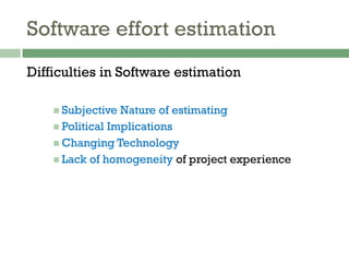
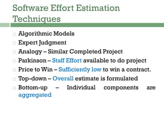
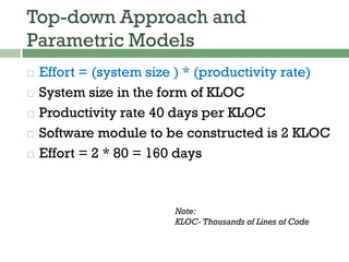
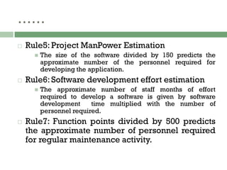
This document discusses various techniques for estimating effort for software projects. It describes common challenges with software estimation like subjective nature and changing requirements. It then explains different estimation techniques like algorithmic models, expert judgment, analogy, top-down and bottom-up approaches. Specifically, it outlines the function point analysis technique and COCOMO model for estimating effort based on source lines of code and complexity factors. Finally, it lists some typical rules of thumb for software estimation from Capers Jones.

1. SOFTWARE PROJECT
MANAGEMENT
Prof. Kanchana Devi V

2. Software Effort Estimation
 Successful project is that the system is
delivered on time and within budget and
with the required quality.

3. Software effort estimation
Difficulties in Software estimation
 Subjective Nature of estimating
 Political Implications
 Changing Technology
 Lack of homogeneity of project experience

4. Project Data
Note:
SLOC - Source Number of Lines of Code
WM -Work in Month

5. Where are estimates done?
 Estimates are carried out at various stages of
software project.
 Strategic Planning
 Decide priority to each project.
 Feasibility Study
 Benefits of potential system
 System Specification
 Detailed requirement analysis at design stage.
 Evaluation of Suppliers Proposals
 Tender Management
 Project Planning
 Detailed estimates of smaller work components during
implementation.

6. Software Effort Estimation
Techniques
 Algorithmic Models
 Expert Judgment
 Analogy – Similar Completed Project
 Parkinson – Staff Effort available to do project
 Price to Win – Sufficiently low to win a contract.
 Top-down – Overall estimate is formulated
 Bottom-up – Individual components are
aggregated

7. Bottom-up Estimating
 Work Breakdown Structure
 Assumptions about characteristics of final
system
 Number and Size of software modules.
 Appropriate at detailed stages of project
planning.
 When a project is completely novel or no
historical data available.

8. Top-down Approach and
Parametric Models
 Effort = (system size ) * (productivity rate)
 System size in the form of KLOC
 Productivity rate 40 days per KLOC
 Software module to be constructed is 2 KLOC
 Effort = 2 * 80 = 160 days
Note:
KLOC- Thousands of Lines of Code

9. Expert Judgment
 Asking for estimate of task effort from
someone who is knowledgeable about either
application or development environment.
 Experts use the combination of informal
analogy approach where similar projects
from past are identified and bottom up
estimating.

10. Estimating by Analogy
 Called “Case Based Analogy”
 Estimator identifies completed projects
source cases with similar characteristics to
new project (target case)
 Effort of the source case used as base
estimate for target.
 TOOL – ANGEL software tool
 Measuring Euclidean Distance between the
cases

11. Euclidean Distance

12. Problems with Over and Under
Estimates
 Parkinson’s Law
 “Given an easy target staff will work less hard”
 Brook’s Law
 Effort required to implement a project will go up
disproportionately with the number of staff assigned
to the project
 “ Putting more people on a late job makes it later”

13. Measure of Work
 Measure such as
 SLOC ( Source Lines of Code)
 KLOC ( Thousand Lines of Code)

14. Albrecht Function Point Analysis
 Top - down method devised by Allan
Albrecht(IBM)
 Developed the idea of Function Points(FPs)
 Basis of function point analysis has five
components:
 External Input Types
 External Output Types
 External Inquiry Types – US spelling inquiry
 Logical Internal File Types – Data store
 External Interface File Types – To & Fro (BACS)
BACS-Bank Automation Clearing System

15. Albrecht Complexity Multipliers

16. IFPUG File Type Complexity

17. Example:
 A logical Internal File contain:
 Purchase order organized into two separate record
types:
 Main purchase order details
 Purchase order number, supplier reference,
purchase order date
 Purchase order item details
 product code, unit price and number ordered.
 No. of record types = 2
 No. of data types = 6
 File type would be rated as low
 FP Count=7

18. Function Points Mark II
 Sponsored by CCTA(Central Computer and
Telecommunications Agency)
 Mark II – Improvement and replacement in
Albrecht method
 In Albrecht method
 Information Processing Size is measured in
UFPs(Unadjusted Functional Points)
 Then TCA(Technical Complexity Adjustment) is
applied

19. Model of Transaction
Data Store
ProcessFrom User Return to
User
Input Output

20. For each transaction UFPs are
calculated
 UFPs = Wi * (number of input data element types)+ We
* (number of entity types referenced)+ Wo * (number of
output data element types)
 Wi We Wo are weightings derived by asking
the developers the proportions of effort
spent.
 FP counters use industry averages which are:
 Wi = 0.58
 We = 1.66
 Wo = 0.26

21. COSMIC Full Function Points
 Cosmic deals with decomposing the system
architecture into hierarchy of software layers.
 Inputs and outputs are aggregated into data
groups
 Each data group brings together data items that
relate to the same object of interest.
 Data Groups can be moved in 4 ways:
 Entries(E)
 Exits(X)
 Reads ( R)
 Writes(W)

22. COCOMO II
 COCOMO (Constructive Cost Model)-Boehm
 Formula :
 (effort)=c(size)k
 Effort measured in pm(number of person-month)
 Size in kdsi (Thousands of delivered source code instructions)
 C,K constants
 C and K are from
System Type C K
Organic 2.4 1.05
Semi-detached 3.0 1.12
Embedded 3.6 1.20

23.  Organic Mode:
 Small teams develop software in a highly
familiar environment (Small & Flexible)
 Embedded Mode:
 Operate within very tight constraints and
changes to the system very costly
 Semi-Detached Mode:
 Combined elements of both

24. COCOMO II - Models
 It has three stages
 Application Composition
 Early Design
 Post Architecture

25. Estimate of person-months
 pm=A(size)(sf)*(em1) *(em2) *(em3)*.. *(emn)
 Pm  Effort in person-months
 A  Constant (In 2000 - 2.94)
 Size  kdsi
 sf  Exponent Scale Factor
 Exponent Scale Factor is derived as
 Sf= B+0.01*∑(Exponent driver ratings)
 B Constant (0.91)

26. Exponent Driver Ratings
 Precedentedness(PREC)
 Development Flexibility(FLEX)
 Risk Resolution(RESL)
 Team Cohesion(TEAM)
 Process Maturity(PMAT)
Driver Very low Low Nominal High Very
High
Extra
High
PREC 6.20 4.96 3.72 2.48 1.24 0.00
FLEX 5.07 4.05 3.04 2.03 1.01 0.00
RESL 7.07 5.65 4.24 2.83 1.41 0.00
TEAM 5.48 4.38 3.29 2.19 1.10 0.00
PMAT 7.80 6.24 4.68 3.12 1.56 0.00

27. Capers Jones Estimating Rules of
Thumb
 Rule1: SLOC Function Point Equivalence
 One Function Point = 125 SLOC For C Programs
 Rule2: Project duration estimation
 Function points raised to the power 0.4 predicts the
approximate development time in calendar months.
 Rule3: Rate of requirements creep
 User requirements creep in at average rate of 2%
per month from the design through coding phases.
 Rule4: Defect Removal Efficiency
 Each software review, inspection, or test step will
find and remove 30% of the bugs that are present

28. ……
 Rule5: Project ManPower Estimation
 The size of the software divided by 150 predicts the
approximate number of the personnel required for
developing the application.
 Rule6: Software development effort estimation
 The approximate number of staff months of effort
required to develop a software is given by software
development time multiplied with the number of
personnel required.
 Rule7: Function points divided by 500 predicts
the approximate number of personnel required
for regular maintenance activity.

29.  http://www.youtube.com/watch?v=9LSnINgl
kQA