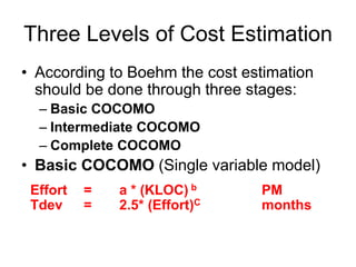
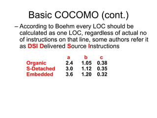
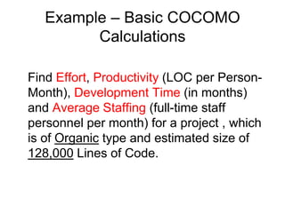
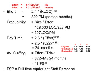
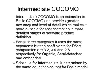
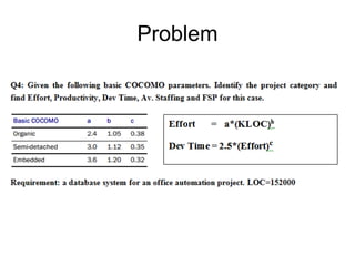
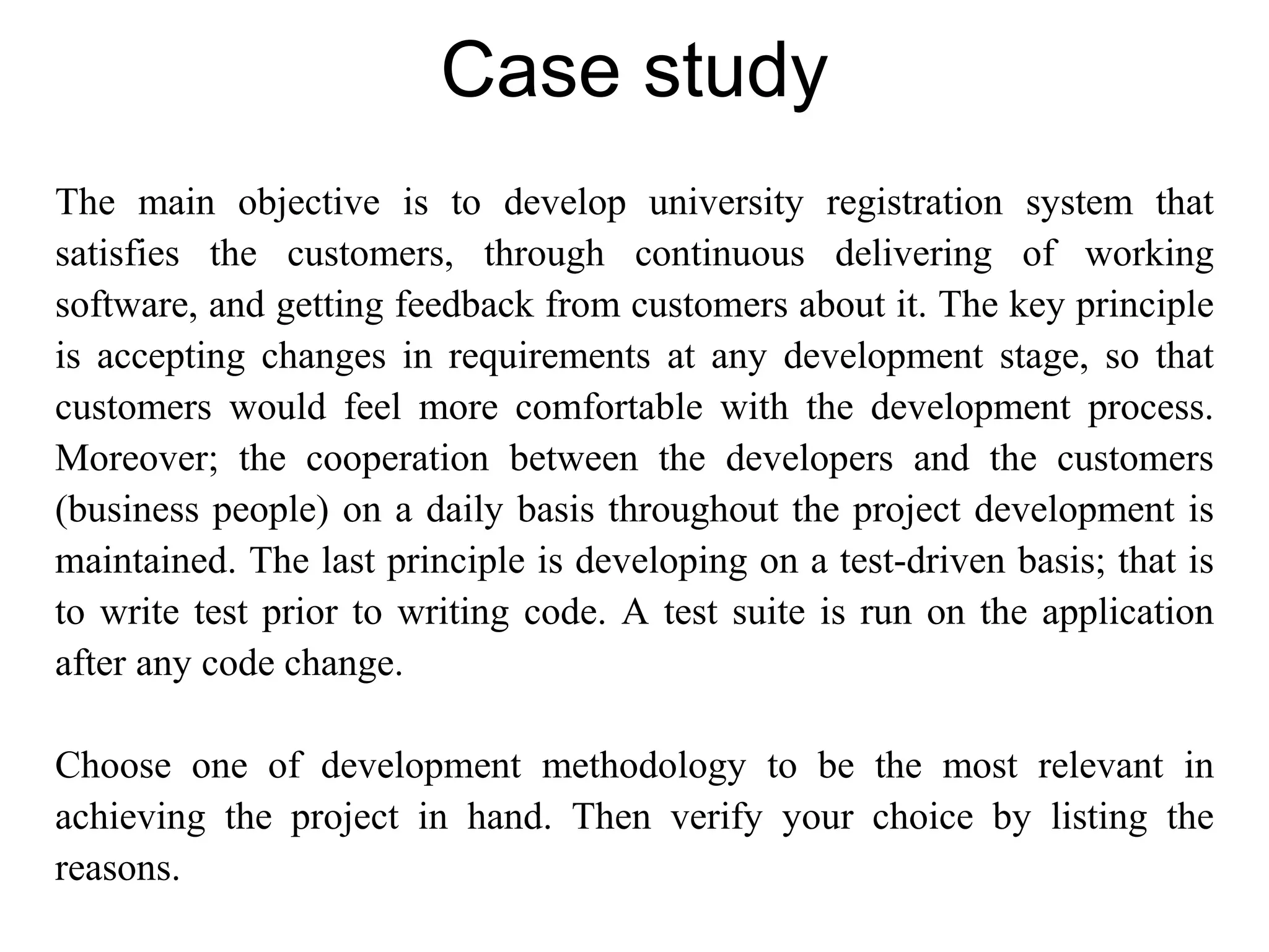
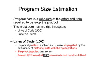
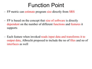
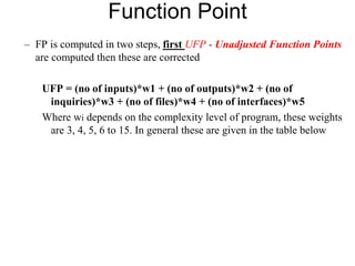
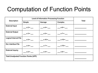
The document outlines the development of a university registration system with a focus on software that meets customer needs through continuous feedback and test-driven development. It details methods for estimating software project size using function points and the COCOMO model for cost and schedule estimation, highlighting various estimation techniques such as empirical, heuristic, and analytical methods. Additionally, it discusses the importance of cooperation between developers and customers throughout the development process, and the influence of environmental factors on project estimation.

1. Case study
The main objective is to develop university registration system that
satisfies the customers, through continuous delivering of working
software, and getting feedback from customers about it. The key principle
is accepting changes in requirements at any development stage, so that
customers would feel more comfortable with the development process.
Moreover; the cooperation between the developers and the customers
(business people) on a daily basis throughout the project development is
maintained. The last principle is developing on a test-driven basis; that is
to write test prior to writing code. A test suite is run on the application
after any code change.
Choose one of development methodology to be the most relevant in
achieving the project in hand. Then verify your choice by listing the
reasons.

2. CS 442
Software Project Management
Project Estimation

3. Program Size Estimation
– Program size is a measure of the effort and time
required to develop the product
– The most common metrics in use are
• Lines of Code (LOC)
• Function Points
– Lines of Code (LOC)
• Historically oldest, evolved and its use propagated by the
availability of historical data with the organizations
• Simplest, popular, and so on
• Source LOC counted BUT comments and headers left out

4. Function Point
– FP metric can estimate program size directly from SRS
– FP is based on the concept that size of software is directly
dependent on the number of different functions and features it
supports
– Each feature when invoked reads input data and transforms it to
output data, Albrecht proposed to include the no of files and no of
interfaces as well

5. Function Point
– FP is computed in two steps, first UFP - Unadjusted Function Points
are computed then these are corrected
UFP = (no of inputs)*w1 + (no of outputs)*w2 + (no of
inquiries)*w3 + (no of files)*w4 + (no of interfaces)*w5
Where wi depends on the complexity level of program, these weights
are 3, 4, 5, 6 to 15. In general these are given in the table below

6. Computation of Function Points
Description
Level of Information Processing Function
Total
Simple Average Complex
External Input
___ x 2 = ___ ___ x 4 = ___ ___ x 6 = ___ _____________
External Output
___ x 3 = ___ ___ x 5 = ___ ___ x 7 = ___ _____________
Logical Internal File
___ x 5 = ___ ___ x 10 =___ ___ x 15 = ___ _____________
Ext. Interface File
___ x 4 = ___ ___ x 7 = ___ ___ x 10 = ___ _____________
External Inquiry
___ x 2 = ___ ___ x 4 = ___ ___ x 6 = ___ _____________
Total Unadjusted Function Points (UFP)
_____________

7. Computation of FP
– In the second step, first Degree of Influence - DI, is
computed considering 14 possible factors, each having
influence value varying from 0 (no influence) to 5
(maximum influence), so DI can vary from 0 - 70
– The parameters considered for DI computation are shown
in the table (on next slide)
– Technical Complexity Factor: TCF is computed using
TCF = 0.65 + 0.01 * DI
– TCF varies from 0.65 to 1.35, and in second step FP is
computed by
FP = UFP * TCF

8. ID Characteristic DI ID Characteristic DI
C1 Data Communications --- C8 On-Line Update ---
C2 Distributed Functions --- C9 Complex Processing ---
C3 Performance --- C10 Re-Usability ---
C4 Heavily Used Configuration --- C11 Installation Ease ---
C5 Transaction Rate --- C12 Operational Ease ---
C6 On-Line Data Entry --- C13 Multiple Sites ---
C7 End User Efficiency --- C14 Facilitate Change ---
Total Degree of Influence
TCF = 0.65 + 0.01 x (Total ‘Degree of Influence’)
FP = UFP * TCF
DI Values
Not Present, or not Influence = 0
Insignificant Influence = 1
Moderate Influence = 2
Average Influence = 3
Significant Influence = 4
Strong Influence, throughout = 5

9. FP Example
Description
Level of Information Processing Function
Total
Simple Average Complex
External Input
3x 2 = 6 4x 4 = 16 1x 6 = 6 28
External Output
0x 3 = 0 6x 5 = 30 2x 7 = 14 44
Logical Internal File
0x 5 = 0 0x 10 =0 5x 15 = 75 75
Ext. Interface File
0x 4 = 0 3x 7 = 21 4x 10 = 40 61
External Inquiry
0x 2 = 0 8x 4 = 32 0x 6 = 0 32
Total Unadjusted Function Points (UFP) 240

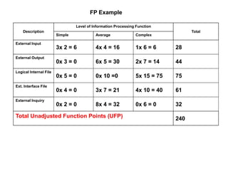
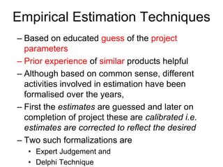
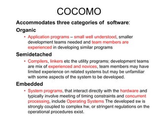
10. Continuing our example . . .
Complex processing = 3
Code to be reusable = 2
High performance = 4
Multiple sites = 3
Distributed processing = 5
Project adjustment factor = 17
Adjustment calculation:
Adjusted FP = Unadjusted FP X [0.65 + (adjustment factor X 0.01)]
= 240 X [0.65 + ( 17 X 0.01)]
= 240 X [0.82]
= 197 Adjusted function points

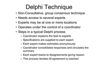
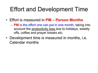
11. Function Point Analysis
But how long will the project take and how much
will it cost?
• As previously measured, programmers in an
organization average 18 function points per
month. Thus . . .
197 FP divided by 18 = 11 man-months
• If the average programmer is paid $5,200 per
month (including benefits), then the [labor] cost
of the project will be . . .
11 man-months X $5,200 = $57,200

12. FP Cons
• Shortcomings
– Allocation of parameters is subjective
– Symons 1988 pointed out that the proposed FP
analysis is based on two ‘intrinsic’ factors but did not
include the Environmental factors like Project
Management Risks, People Skills, Methods and
tools used for development etc
• His proposed method includes the influence of
Environmental factors
– Algorithmic complexity not taken into account

13. Project Estimation Techniques
– After determining the Project Size; effort to
develop the sw, project duration and cost are
to be estimated
– These parameters help in winning the
contract, as well as in resource planning,
scheduling, monitoring and controlling the
project
– Estimation Techniques can be categorised as:
• Empirical Estimation Techniques
• Heuristic Techniques
• Analytical Estimation Techniques

14. Empirical Estimation Techniques
– Based on educated guess of the project
parameters
– Prior experience of similar products helpful
– Although based on common sense, different
activities involved in estimation have been
formalised over the years,
– First the estimates are guessed and later on
completion of project these are calibrated i.e.
estimates are corrected to reflect the desired
– Two such formalizations are
• Expert Judgement and
• Delphi Technique

15. Delphi Technique
• Non-Consultative, group consensus technique
• Needs access to several experts
• Experts may be at one or more locations
• Operates under the control of a coordinator
• Steps in a typical Delphi process
– Coordinator explains the task to experts
– Specifications are supplied to each expert
– Each expert makes estimates anonymously
– Coordinator consolidates responses and circulates the
summary
– Each expert reacts to disagreements giving reason
– This process iterates till agreement is reached

16. Heuristic Techniques
– Assumes that relationships among the
different project parameters can be modelled
using suitable mathematical expressions
– Once basic (independent) parameters are
known,the other (dependent) parameters can
be determined using basic parameters in
mathematical expressions
– Heuristic Models can be divided into two
classes:
• Single variable estimation models
• Multivariable estimation models

17. COCOMO
• COCOMO
COnstructive COst-estimation MOdel
– A software cost and schedule estimating
method
– developed by Barry W Boehm.
– The model is an empirically derived, based
on a study by Boehm of 63 sw
development projects.

18. COCOMO
Accommodates three categories of software:
Organic
• Application programs – small well understood, smaller
development teams needed and team members are
experienced in developing similar programs
Semidetached
• Compilers, linkers etc the utility programs; development teams
are mix of experienced and novices, team members may have
limited experience on related systems but may be unfamiliar
with some aspects of the system to be developed.
Embedded
• System programs, that interact directly with the hardware and
typically involve meeting of timing constraints and concurrent
processing, include Operating Systems The developed sw is
strongly coupled to complex hw, or stringent regulations on the
operational procedures exist.

19. Effort and Development Time
• Effort is measured in PM – Person Months
– PM is the effort one can put in one month, taking into
account the productivity loss due to holidays, weekly
offs, coffee and prayer breaks etc.
• Development time is measured in months, i.e.
Calendar months

20. Three Levels of Cost Estimation
• According to Boehm the cost estimation
should be done through three stages:
– Basic COCOMO
– Intermediate COCOMO
– Complete COCOMO
• Basic COCOMO (Single variable model)
Effort = a * (KLOC) b PM
Tdev = 2.5* (Effort)C months

21. Basic COCOMO (cont.)
– According to Boehm every LOC should be
calculated as one LOC, regardless of actual no
of instructions on that line, some authors refer it
as DSI Delivered Source Instructions
a b c
Organic 2.4 1.05 0.38
S-Detached 3.0 1.12 0.35
Embedded 3.6 1.20 0.32

22. Example – Basic COCOMO
Calculations
Find Effort, Productivity (LOC per Person-
Month), Development Time (in months)
and Average Staffing (full-time staff
personnel per month) for a project , which
is of Organic type and estimated size of
128,000 Lines of Code.

23. • Effort = 2.4 * (KLOC)1.05
= 322 PM (person-months)
• Productivity = Size / Effort
= 128,000 LOC/322 PM
= 397LOC/PM
• Dev Time = 2.5 * (Effort)0.38
= 2.5 * (322) 0.38
= 24 months
• Av. Staffing = Effort / Tdev
= 322PM / 24 months
= 16 FSP
• FSP = Full time equivalent Staff Personnel
a b c
Organic 2.4 1.05 0.38
S-Detached 3.0 1.12 0.35
Embedded 3.6 1.20 0.32
Effort = a * (KLOC) b PM
Tdev = 2.5* (Effort)C months

24. Intermediate COCOMO
– Intermediate COCOMO is an extension to
Basic COCOMO and provides greater
accuracy and level of detail which makes it
more suitable for cost estimation in more
detailed stages of software product
definition.
– For all three categories it uses the same
exponents but the coefficients for Effort
computation are 3.2, 3.0 and 2.8
respectively for Organic, Semi-detached
and embedded.
– Schedule for Intermediate is determined by
the same equations as that for Basic model

25. Problem