Downloaded 120 times


![Bottom-up estimating
1. Break project into smaller and smaller
components
[2. Stop when you get to what one person can
do in one/two weeks]
3. Estimate costs for the lowest level activities
4. At each higher level calculate estimate by
adding estimates for lower levels
6](https://image.slidesharecdn.com/17912chapter05softwareeffortestimation-140323143410-phpapp02/85/software-effort-estimation-6-320.jpg)

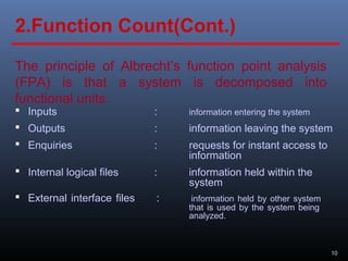
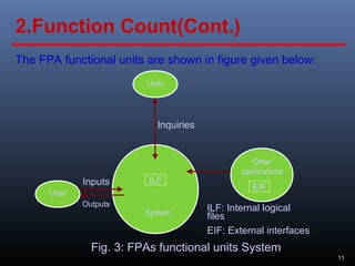
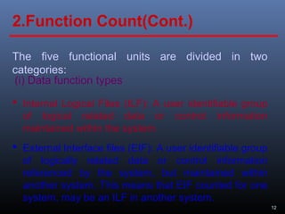
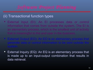
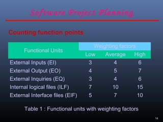
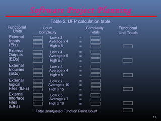
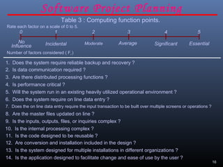
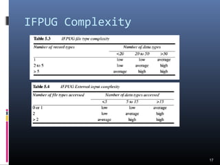
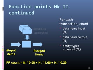
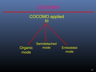
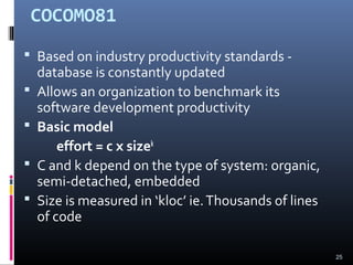
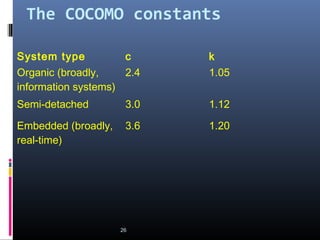
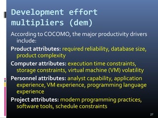
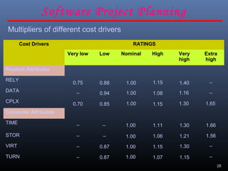
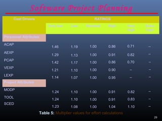
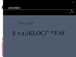

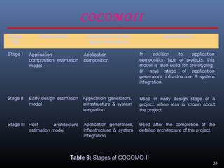

A document discusses various software estimation techniques including function point analysis, COCOMO models, and cost drivers. Function point analysis breaks a system into functional components like inputs, outputs, inquiries and files that are assigned complexity weights and counts. COCOMO models like COCOMO I and COCOMO II estimate effort using size of the project and cost multipliers related to attributes of the product, computer system, personnel and project. Cost drivers help assess these multipliers to refine effort estimates.