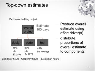
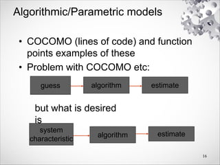
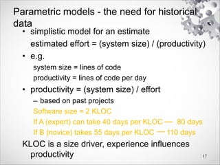
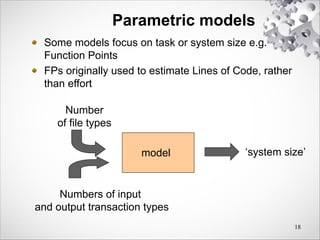
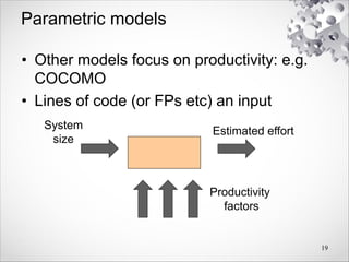
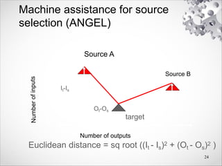
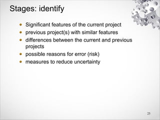
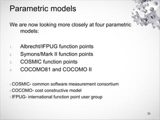
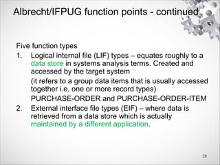
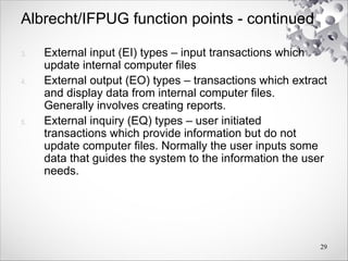
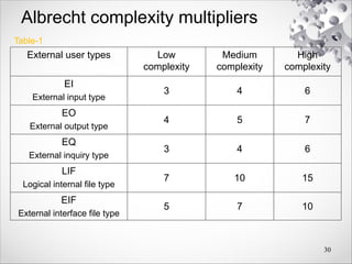
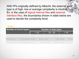
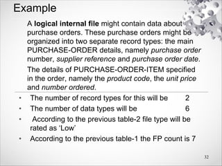
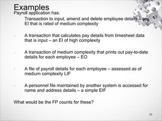
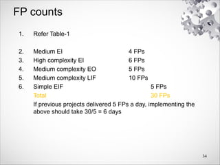
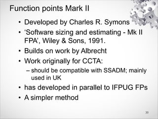
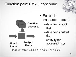
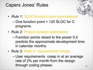
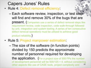
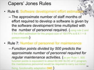
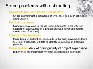
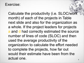
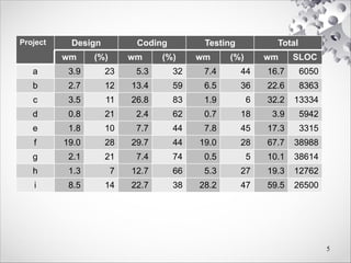
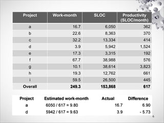
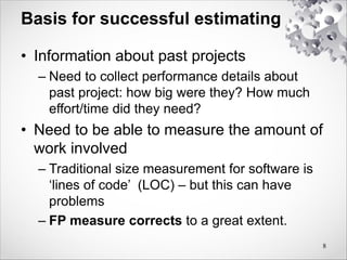
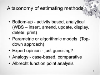
Chapter five discusses the complexities and challenges in software effort estimation, emphasizing the need for accurate predictions to meet project targets effectively. It highlights various factors influencing estimates, including political pressures, changing technologies, and individual project differences, while suggesting methods like bottom-up and top-down estimating approaches alongside function point analysis. Additionally, it addresses the importance of leveraging data from past projects to enhance the reliability and accuracy of future estimates.

1. Software Project Management
Chapter Five
Software effort estimation
1
Software project management (5e) - introduction © The McGraw-Hill Companies, 2011

2. What makes a successful project?
Delivering:
• agreed functionality
• on time
• at the agreed cost
• with the required quality
Stages:
1. set targets
2. Attempt to achieve
targets
2
BUT what if the targets are not achievable?
Difficulties in estimating due to complexity and invisibility of software.

3. Some problems with estimating
• Subjective nature of much of estimating
– Under estimating the difficulties of small task and over estimating
large projects.
• Political pressures
– Managers may wish to reduce estimated costs in order to win
support for acceptance of a project proposal (over estimate to
create a comfort zone)
• Changing technologies
– these bring uncertainties, especially in the early days when there
is a ‘learning curve’. Difficult to use the experience of previous
projects.
• Projects differ -lack of homogeneity of project experience
– Experience on one project may not be applicable to another
3

4. Exercise:
Calculate the productivity (i.e. SLOC/work
month) of each of the projects in Table
next slide and also for the organization as
a whole. If the project leaders for projects
a and d had correctly estimated the source
number of lines of code (SLOC) and then
used the average productivity of the
organization to calculate the effort needed
to complete the projects, how far out
would their estimate have been from the
actual one. 4

5. Project Design Coding Testing Total
wm (%) wm (%) wm (%) wm SLOC
a 3.9 23 5.3 32 7.4 44 16.7 6050
b 2.7 12 13.4 59 6.5 36 22.6 8363
c 3.5 11 26.8 83 1.9 6 32.2 13334
d 0.8 21 2.4 62 0.7 18 3.9 5942
e 1.8 10 7.7 44 7.8 45 17.3 3315
f 19.0 28 29.7 44 19.0 28 67.7 38988
g 2.1 21 7.4 74 0.5 5 10.1 38614
h 1.3 7 12.7 66 5.3 27 19.3 12762
i 8.5 14 22.7 38 28.2 47 59.5 26500
5

6. Project Work-month SLOC Productivity
(SLOC/month)
a 16.7 6,050 362
b 22.6 8,363 370
c 32.2 13,334 414
d 3.9 5,942 1,524
e 17.3 3,315 192
f 67.7 38,988 576
g 10.1 38,614 3,823
h 19.3 12,762 661
i 59.5 26,500 445
Overall
6

7. Over and under-estimating
• Parkinson’s Law:
‘Work expands to fill
the time available’
• An over-estimate is
likely to cause project
to take longer than it
would otherwise
• Weinberg’s Zeroth Law
of reliability: ‘a software
project that does not
have to meet a
reliability requirement
can meet any other
requirement’
7
• Brook’s Law: ‘putting more people on a late job
makes it later’. If there is an overestimate of the
effort required, this could lead to more staff being
allocated than needed and managerial overheads
being increased.

8. Basis for successful estimating
• Information about past projects
– Need to collect performance details about
past project: how big were they? How much
effort/time did they need?
• Need to be able to measure the amount of
work involved
– Traditional size measurement for software is
‘lines of code’ (LOC) – but this can have
problems
– FP measure corrects to a great extent.
8

9. A taxonomy of estimating methods
• Bottom-up - activity based, analytical
(WBS – insert, amend, update, display,
delete, print)
• Parametric or algorithmic models (Top-
down approach)
• Expert opinion - just guessing?
• Analogy - case-based, comparative
• Albrecht function point analysis
9

10. Parameters to be Estimated
• Size is a fundamental measure of work
• Based on the estimated size, two
parameters are estimated:
– Effort
– Duration
• Effort is measured in person-months:
– One person-month is the effort an individual
can typically put in a month.
10

11. Measure of Work
• The project size is a measure of the
problem complexity in terms of the effort
and time required to develop the product.
• Two metrics are used to measure project
size:
– Source Lines of Code (SLOC)
– Function point (FP)
• FP is now-a-days favored over SLOC:
– Because of the many shortcomings of SLOC.
11

12. Major Shortcomings of SLOC
• No precise definition (e.g. comment
line, data declaration line to be
included or not?)
• Difficult to estimate at start of a project
• Only a code measure
• Programmer-dependent
• Does not consider code complexity
12

13. Bottom-up versus top-down
• Bottom-up
– use when no past project data
– identify all tasks that have to be done – so
quite time-consuming
– use when you have no data about similar
past projects
• Top-down
– produce overall estimate based on project
cost drivers
– based on past project data
– divide overall estimate between jobs to be
done 13

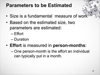
14. Bottom-up estimating
1. Break project into smaller and smaller components
2. Stop when you get to what one person can do in
one/two weeks]
3. Estimate costs for the lowest level activities
4. At each higher level calculate estimate by adding
estimates for lower levels
A procedural code-oriented approach
a) Envisage the number and type of modules in the
final system
b) Estimate the SLOC of each individual module
c) Estimate the work content
d) Calculate the work-days effort
14

15. Top-down estimates
• Produce overall
estimate using
effort driver(s)
• distribute
proportions of
overall estimate
to components
15
design code
overall
project
test
Estimate
100 days
30%
i.e.
30 days
30%
i.e.
30 days
40%
i.e. 40 days
Normally associated with parametric (or algorithmic) model.
Ex: House building project
Bick-layer hours Carpentry hours Electrician hours

16. Algorithmic/Parametric models
• COCOMO (lines of code) and function
points examples of these
• Problem with COCOMO etc:
16
guess algorithm estimate
but what is desired
is
system
characteristic
algorithm estimate

17. Parametric models - the need for historical
data
• simplistic model for an estimate
estimated effort = (system size) / (productivity)
• e.g.
system size = lines of code
productivity = lines of code per day
• productivity = (system size) / effort
– based on past projects
Software size = 2 KLOC
If A (expert) can take 40 days per KLOC 80 days
If B (novice) takes 55 days per KLOC 110 days
KLOC is a size driver, experience influences
productivity 17

18. 18
Parametric models
Some models focus on task or system size e.g.
Function Points
FPs originally used to estimate Lines of Code, rather
than effort
model
Number
of file types
Numbers of input
and output transaction types
‘system size’

19. Parametric models
• Other models focus on productivity: e.g.
COCOMO
• Lines of code (or FPs etc) an input
19
System
size
Productivity
factors
Estimated effort

20. Expert judgement
• Asking someone who is familiar with and
knowledgeable about the application area and
the technologies to provide an estimate
• Particularly appropriate where existing code is to
be modified
• Research shows that experts judgement in
practice tends to be based on analogy
Note: Delphi technique – group decision making
20

21. Estimating by analogy
(Case-based reasoning)
21
source cases-completed projects
attribute values
effort
attribute values ?????
target case (new)
attribute values
attribute values
attribute values
attribute values
attribute values
effort
effort
effort
effort
effort Select case
with closet attribute
values
Use effort adjustment
from source as estimate

22. Estimating by analogy…cont.
• Use of ANGEL software tool (measure the Euclidean
distance between project cases)
• Example:
Say that the cases are being matched on the basis of
two parameters, the number of inputs to and the
number of outputs from the application to be built.
The new project is known to require 7 inputs and 15
outputs. One of the past cases, project A, has 8
inputs and 17 outputs.
The Euclidian distance between the source and the
target is therefore
= 2.24
22
)
)
15
17
(
)
8
7
(( 2
2



)
)
15
17
(
)
8
7
(( 2
2




23. Exercise:
Project B has 5 inputs and 10 outputs. What would
be the Euclidian distance between this project and
the target new project being considered in the
previous slide? Is project B a better analogy with the
target than project A?
The Euclidian distance between project B and the
target case is = 5.39.
Therefore project A is a closer analogy.
23
)
)
10
15
(
)
5
7
(( 2
2




24. Machine assistance for source
selection (ANGEL)
24
Nu
mb
er
of
inp
uts
Number of outputs
target
Source A
Source B
Euclidean distance = sq root ((It - Is)2 + (Ot - Os)2 )
It-Is
Ot-Os

25. Stages: identify
Significant features of the current project
previous project(s) with similar features
differences between the current and previous
projects
possible reasons for error (risk)
measures to reduce uncertainty
25

26. Parametric models
We are now looking more closely at four parametric
models:
1. Albrecht/IFPUG function points
2. Symons/Mark II function points
3. COSMIC function points
4. COCOMO81 and COCOMO II
5.COSMIC- common software measurement consortium
6.COCOMO- cost constructive model
7.IFPUG- international function point user group
26

27. Albrecht/IFPUG function points
• Albrecht worked at IBM and needed a way of
measuring the relative productivity of different
programming languages.
• Needed some way of measuring the size of
an application without counting lines of code.
• Identified five types of component or
functionality in an information system
• Counted occurrences of each type of
functionality in order to get an indication of
the size of an information system
Note: IFPUG- International FP User Group
27

28. Albrecht/IFPUG function points - continued
Five function types
1. Logical internal file (LIF) types – equates roughly to a
data store in systems analysis terms. Created and
accessed by the target system
(it refers to a group data items that is usually accessed
together i.e. one or more record types)
PURCHASE-ORDER and PURCHASE-ORDER-ITEM
2. External interface file types (EIF) – where data is
retrieved from a data store which is actually
maintained by a different application.
28

29. Albrecht/IFPUG function points - continued
3. External input (EI) types – input transactions which
update internal computer files
4. External output (EO) types – transactions which extract
and display data from internal computer files.
Generally involves creating reports.
5. External inquiry (EQ) types – user initiated
transactions which provide information but do not
update computer files. Normally the user inputs some
data that guides the system to the information the user
needs.
29

30. Albrecht complexity multipliers
External user types Low
complexity
Medium
complexity
High
complexity
EI
External input type
3 4 6
EO
External output type
4 5 7
EQ
External inquiry type
3 4 6
LIF
Logical internal file type
7 10 15
EIF
External interface file type
5 7 10
30
Table-1

31. With FPs originally defined by Albecht, the external user
type is of high, low or average complexity is intuitive.
Ex: in the case of logical internal files and external
interface files, the boundaries shown in table below are
used to decide the complexity level.
Number of record types Number of data types
< 20 20 – 50 > 50
1 Low Low Average
2 to 5 Low Average High
> 5 Average High High
31
Table-2

32. Example
A logical internal file might contain data about
purchase orders. These purchase orders might be
organized into two separate record types: the main
PURCHASE-ORDER details, namely purchase order
number, supplier reference and purchase order date.
The details of PURCHASE-ORDER-ITEM specified
in the order, namely the product code, the unit price
and number ordered.
• The number of record types for this will be 2
• The number of data types will be 6
• According to the previous table-2 file type will be
rated as ‘Low’
• According to the previous table-1 the FP count is 7
32

33. Examples
Payroll application has:
1. Transaction to input, amend and delete employee details – an
EI that is rated of medium complexity
2. A transaction that calculates pay details from timesheet data
that is input – an EI of high complexity
3. A transaction of medium complexity that prints out pay-to-date
details for each employee – EO
4. A file of payroll details for each employee – assessed as of
medium complexity LIF
5. A personnel file maintained by another system is accessed for
name and address details – a simple EIF
What would be the FP counts for these?
33

34. FP counts
1. Refer Table-1
2. Medium EI 4 FPs
3. High complexity EI 6 FPs
4. Medium complexity EO 5 FPs
5. Medium complexity LIF 10 FPs
6. Simple EIF 5 FPs
Total 30 FPs
If previous projects delivered 5 FPs a day, implementing the
above should take 30/5 = 6 days
34

35. Function points Mark II
• Developed by Charles R. Symons
• ‘Software sizing and estimating - Mk II
FPA’, Wiley & Sons, 1991.
• Builds on work by Albrecht
• Work originally for CCTA:
– should be compatible with SSADM; mainly
used in UK
• has developed in parallel to IFPUG FPs
• A simpler method
35

36. Function points Mk II continued
• For each
transaction, count
– data items input
(Ni)
– data items output
(No)
– entity types
accessed (Ne)
36
#entities
accessed
#input
items
#output
items
FP count = Ni * 0.58 + Ne * 1.66 + No * 0.26

37. • UFP – Unadjusted Function Point – Albrecht
(information processing size is measured)
• TCA – Technical Complexity Adjustment
(the assumption is, an information system
comprises transactions which have the basic
structures, as shown in previous slide)
• For each transaction the UFPs are calculated:
Wi X (number of input data element types) +
We X (number of entity types referenced) +
Wo X (number of output data element types)
Wi ,We ,Wo are weightings derived by asking
developers the proportions of effort spent in previous
projects developing the code dealing with input,
accessing stored data and outputs.
Wi = 0.58, We = 1.66, Wo = 0.26 (industry average)
37

38. Exercise:
A cash receipt transaction in an accounts subsystem
accesses two entity types INVOICE and CASH-RECEIPT.
The data inputs are:
Invoice number
Date received
Cash received
If an INVOICE record is not found for the invoice number
then an error message is issued. If the invoice number is
found then a CASH-RECEIPT record is created. The error
message is the only output of the transaction. Calculate
the unadjusted function points, using industry average
weightings, for this transaction. Ne=2, Ni=3, No=1
(0.58 X 3) + (1.66 X 2) + (0.26 X 1) = 5.32
38

39. Exercise:
In an annual maintenance contract subsystem is having a
transaction which sets up details of new annual
maintenance contract customers.
1. Customer account number 2.Customer name
3. Address 4. Postcode
5. Customer type 6. Renewal date
All this information will be set up in a CUSTOMER record
on the system’s database. If a CUSTOMER account
already exists for the account number that has been input,
an error message will be displayed to the operator.
Calculate the number of unadjusted Mark II function points
for the transaction described above using the industry
average.
39

40. Answer:
The function types are:
Input data types 6
Entities accessed 1
Output data types 1
UFP = Unadjusted function points
= (0.58 X 6) + (1.66 X 1) + (0.26 X 1)
= 5.4
40

41. Function points for embedded systems
Mark II function points, IFPUG function points were
designed for information systems environments
They are not helpful for sizing real-time or embedded
systems
COSMIC-FFPs (common software measurement
consortium-full function point) attempt to extend
concept to embedded systems or real-time systems
FFP method origins the work of two interlinked
groups in Quebec, Canada
Embedded software seen as being in a particular
‘layer’ in the system
Communicates with other layers and also other
components at same level
41

42. The argument is
• existing function point method is
effective in assessing the work content
of an information system.
• size of the internal procedures mirrors
the external features.
• in real-time or embedded system, the
features are hidden because the
software’s user will probably not be
human beings but a hardware device.
42

43. • COSMIC deals with by decomposing the
system architecture into a hierarchy of
software layers.
• The software component to be sized can
receive requests the service from layers
above and can request services from those
below.
• There may be separate software components
engage in peer-to-peer communication.
• Inputs and outputs are aggregated into data
groups, where each data group brings
together data items related to the same
objects. 43

44. Layered software
44
Higher layers
Lower layers
Software component peer
component
Makes a request
for a service
Receives service
Receives request Supplies service
Peer to peer
communication
Persistent
storage
Data reads/
writes

45. COSMIC FPs
The following are counted:
(Data groups can be moved in four ways)
Entries (E): movement of data into software
component from a higher layer or a peer component
Exits (X): movements of data out to a user outside
its boundary
Reads (R): data movement from persistent storage
Writes (W): data movement to persistent storage
Each counts as 1 ‘COSMIC functional size unit’ (Cfsu). The
overall FFP count is derived by simply adding up the
counts for each of the four types of data movement.
45

46. Exercise:
A small computer system controls the entry of vehicles
to a car park. Each time a vehicle pulls up before an
entry barrier, a sensor notifies the computer system of
the vehicle’s presence. The system examines a count
that it maintains the number of vehicles currently in the
car park. This count is kept on the backing storage so
that it will still be available if the system is temporarily
shut down, for example because of a power cut. If the
count does not exceed the maximum allowed then the
barrier is lifted and count is incremented. When the
vehicle leaves the car park, a sensor detects the exit
and reduce the count of vehicles.
Identify the entries, exits, reads and writes in this
application.
46

47. 47
Data movement Type
Incoming vehicles sensed
Access vehicle count
Signal barrier to be lifted
Increment vehicle count
Outgoing vehicle sensed
Decrement vehicle count
New maximum input
Set new maximum
Adjust current vehicle count
Record adjusted vehicle count

48. Data movement Type
Incoming vehicles sensed E
Access vehicle count R
Signal barrier to be lifted X
Increment vehicle count W
Outgoing vehicle sensed E
Decrement vehicle count W
New maximum input E
Set new maximum W
Adjust current vehicle count E
Record adjusted vehicle count W
48
Note: different interpretations of the requirements could lead to
different counts. The description in the exercise does not specify to
give a message that the car park is full or has spaces.

49. COCOMO81
Based on industry productivity standards - database is
constantly updated
Allows an organization to benchmark its software
development productivity
Basic model
effort = c x sizek
C and k depend on the type of system: organic, semi-
detached, embedded
Size is measured in ‘kloc’ ie. Thousands of lines of code
Boehm in 1970, on a study of 63 projects, made this model.
Of these only seven were business systems and so the
model was based on other applications (non-information
systems).
49

50. The COCOMO constants
System type c k
Organic (broadly, information systems, small
team, highly familiar in-house environment) 2.4 1.05
Semi-detached (combined characteristics
between organic and embedded modes)
3.0 1.12
Embedded (broadly, real-time, products
developed has to operate within very tight
constraints and changes to system is very costly)
3.6 1.20
50
k exponentiation – ‘to the power of…’
adds disproportionately more effort to the larger projects
takes account of bigger management overheads

51. effort = c (size)k
effort – pm (person month) – 152 working hours
size – KLOC – kdsi (thousands of delivered source
code instruction)
c and k – constants depending on whether the system
is organic, semi-detached or embedded.
Organic : Effort = 2.4(KLOC)1.05 PM
Semidetached : Effort = 3.0(KLOC)1.12 PM
Embedded : Effort = 3.6(KLOC)1.20 PM
51

52. Estimation of development time
Tdev = a X (Effort)b
Organic : 2.5(Effort)0.38
Semidetached : 2.5(Effort)0.35
Embedded : 2.5(Effort)0.32
52

53. Embedded
Semi-detached
Organic
Estimated
effort
Size
Embedded
Semi-detached
Organic
Nominal
development
time
Size
Effort vs. product size
(effort is super-linear in the size of the software)
Effort required to develop a product increases very
rapidly with project size.
Development time vs. product size
(development time is a sub-linear function of the size of the product)
When the size of the software increases by two times,
the development time increases moderately
53

54. Exercise:
Assume that the size of an organic type software
product is estimated to be 32,000 lines of source
code. Assume that the average salary of a software
developer is Rs.50,000 per month. Determine the
effort required to develop the software product, the
nominal development time, and the staff cost to
develop the product.
Effort = 2.4 X 321.05 = 91 pm
Nominal development time = 2.5 X 910.38 = 14 months
Staff cost required to develop the product
91 X Rs. 50,000 = Rs. 45,50,000
54

55. Ex-Two software managers separately estimated a given product to
be of 10,000 and 15,000 lines of code respectively. Bring out the
effort and schedule time implications of their estimation using
COCOMO. For the effort estimation, use a coefficient value of 3.2
and exponent value of 1.05. For the schedule time estimation, the
similar values are 2.5 and 0.38 respectively. Assume all
adjustment multipliers to be equal to unity.
For 10,000 LOC
Effort = 3.2 X 101.05 = 35.90 PM
Schedule Time = Tdev = 2.5 X 35.900.38 = 9.75 months
For 15,000 LOC
Effort = 3.2 X 151.05 = 54.96 PM
Schedule Time = Tdev = 2.5 X 54.960.38 = 11.46 months
NB: Increase in size drastic increase in effort but moderate change in time.
55

56. COCOMO II
An updated version of COCOMO:
• There are different COCOMO II models for estimating at
the ‘early design’ stage and the ‘post architecture’ stage
when the final system is implemented. We’ll look
specifically at the first.
• The core model is:
pm = A(size)(sf) ×(em1) ×(em2) ×(em3)….
where pm = person months, A is 2.94, size is
number of thousands of lines of code, sf is the
scale factor, and em is an effort multiplier
sf = B + 0.01 X Σ (exponent driver ratings)
56

57. COCOMO II Scale factor
Boehm et al. have refined a family of cost estimation
models. The key one is COCOMO II. It uses multipliers and
exponent values. Based on five factors which appear to be
particularly sensitive to system size.
1. Precedentedness (PREC). Degree to which there are
past examples that can be consulted, else uncertainty
2. Development flexibility (FLEX). Degree of flexibility that
exists when implementing the project
3. Architecture/risk resolution (RESL). Degree of
uncertainty about requirements, liable to change
4. Team cohesion (TEAM). Large dispersed
5. Process maturity (PMAT) could be assessed by CMMI,
more structured less uncertainty
6. – see Section 13.8
57

58. COCOMO II Scale factor values
Driver Very low Low Nominal High Very high Extra high
PREC 6.20 4.96 3.72 2.48 1.24 0.00
FLEX 5.07 4.05 3.04 2.03 1.01 0.00
RESL 7.07 5.65 4.24 2.83 1.41 0.00
TEAM 5.48 4.38 3.29 2.19 1.10 0.00
PMAT 7.80 6.24 4.68 3.12 1.56 0.00
58

59. Example of scale factor
• A software development team is
developing an application which is very
similar to previous ones it has developed.
• A very precise software engineering
document lays down very strict
requirements. PREC is very high (score
1.24).
• FLEX is very low (score 5.07).
• The good news is that these tight
requirements are unlikely to change
(RESL is high with a score 2.83).
• The team is tightly knit (TEAM has high 59

60. Scale factor calculation
The formula for sf is
sf = B + 0.01 × Σ scale factor values
i.e. sf = 0.91 + 0.01 × (1.24 + 5.07 +
2.83 + 2.19 + 6.24)
= 1.0857
If system contained 10 kloc then estimate
would be effort = c (size)k = 2.94 x
101.0857 = 35.8 person-months
Using exponentiation (‘to the power of’) adds
disproportionately more to the estimates for
60

61. Exercise:
A new project has ‘average’ novelty for the software supplier
that is going to execute it and thus given a nominal rating on
this account for precedentedness. Development flexibility is
high, requirements may change radically and so risk
resolution exponent is rated very low. The development team
are all located in the same office and this leads to team
cohesion being rated as vey high, but the software house as
a whole tends to be very informal in its standards and
procedures and the process maturity driver has therefore
been given a rating of ‘low’.
(i) (i) What would be the scale factor (sf) in this case?
(ii) (ii) What would the estimate effort if the size of the
application was estimated as in the region of 2000 lines of
code?
61

62. Factor Rating Value
PREC nominal 3.72
FLEX high 2.03
RESL very low 7.07
TEAM very high 1.10
PMAT low 6.24
62
Assessing the scale factors
(i) The overall scale factor = sf = B + 0.01 X Σ (exponent factors)
= 0.91 + 0.01 X (3.72 + 2.03 + 7.07 + 1.10 + 6.24
= 0.91 + 0.01 X 20.16 = 1.112
(ii) The estimated effort = c (size)k = 2.94 X 21.112 = 6.35 staff-months

63. Effort multipliers
(COCOMO II - early design)
As well as the scale factor effort multipliers are also
assessed:
RCPX Product reliability and complexity
RUSE Reuse required
PDIF Platform difficulty
PERS Personnel capability
PREX Personnel experience
FCIL Facilities available
SCED Schedule pressure
63

64. Effort multipliers
(COCOMO II - early design)
Extra
low
Very
low
Low Nom-
inal
High Very
high
Extra
high
RCPX 0.49 0.60 0.83 1.00 1.33 1.91 2.72
RUSE 0.95 1.00 1.07 1.15 1.24
PDIF 0.87 1.00 1.29 1.81 2.61
PERS 2.12 1.62 1.26 1.00 0.83 0.63 0.50
PREX 1.59 1.33 1.12 1.00 0.87 0.74 0.62
FCIL 1.43 1.30 1.10 1.00 0.87 0.73 0.62
SCED 1.43 1.14 1.00 1.00 1.00
64
Table-3

65. Example
• Say that a new project is similar in most
characteristics to those that an
organization has been dealing for some
time
• except
– the software to be produced is exceptionally
complex and will be used in a safety critical
system.
– The software will interface with a new
operating system that is currently in beta
status.
– To deal with this the team allocated to the job 65

66. Example -continued
Refer Table-3
RCPX very high 1.91
PDIF very high 1.81
PERS extra high 0.50
PREX nominal 1.00
All other factors are nominal
Say estimate is 35.8 person months
With effort multipliers this becomes 35.8 x
1.91 x 1.81 x 0.5
= 61.9 person months
66

67. Exercise:
A software supplier has to produce an application that controls a
piece of equipment in a factory. A high degree of reliability is
needed as a malfunction could injure the operators. The
algorithms to control the equipment are also complex. The product
reliability and complexity are therefore rates as very high. The
company would lie to take opportunity to exploit fully the
investment that they made in the project by reusing the control
system, with suitable modifications, on future contracts. The
reusability requirement is therefore rate as very high. Developers
are familiar with the platform and the possibility of potential
problems in that respect is regarded as low. The current staff are
generally very capable and are rated as very high, but the project
is in a somewhat novel application domain for them so experience
s rated as nominal. The toolsets available to the developers are
judged to be typical for the size of company and are rated
nominal, as it is the degree of schedule pressure to meet a
deadline. 67

68. Given the data table-3
(i) What would be the value for each of the effort
multipliers?
(ii) What would be the impact of all the effort multipliers
on a project estimated as taking 200 staff members?
68

69. Factor Description Rating Effort multiplier
RCPX Product reliability and complexity
RUSE Reuse
PDIF Platform difficulty
PERS Personnel capability
PREX Personnel experience
FCIL Facilities available
SCED Required development schedule
69

70. Factor Description Rating Effort multiplier
RCPX Product reliability and complexity Very high
RUSE Reuse Very high
PDIF Platform difficulty Low
PERS Personnel capability Very high
PREX Personnel experience Nominal
FCIL Facilities available Nominal
SCED Required development schedule nominal
70

71. Factor Description Rating Effort multiplier
RCPX Product reliability and complexity Very high 1.91
RUSE Reuse Very high 1.15
PDIF Platform difficulty Low 0.87
PERS Personnel capability Very high 0.63
PREX Personnel experience Nominal 1.00
FCIL Facilities available Nominal 1.00
SCED Required development schedule nominal 1.00
71

72. New development effort multipliers (dem)
According to COCOMO, the major productivity drivers
include:
Product attributes: required reliability, database size,
product complexity
Computer attributes: execution time constraints,
storage constraints, virtual machine (VM) volatility
Personnel attributes: analyst capability, application
experience, VM experience, programming language
experience
Project attributes: modern programming practices,
software tools, schedule constraints
72

73. Modifier type Code Effort multiplier
Product attributes RELY Required software reliability
DATA Database size
DOCU Documentation match to life-cycle needs
CPLX Product complexity
REUSE Required reusability
Platform attributes TIME Execution time constraint
STOR Main storage constraint
PVOL Platform volatility
Personnel attributes ACAP Analyst capability
AEXP Application experience
PCAP Programmer capabilities
PEXP Platform experience
LEXP Programming language experience
PCON Personnel continuity
Project attributes TOOL Use of software tools
SITE Multisite development
SCED Schedule pressure 73
COCOMO
II
Post
architecture
effort
multipliers

74. Staffing
• Norden was one of the first to
investigate staffing pattern:
– Considered general research and
development (R&D) type of projects for
efficient utilization of manpower.
• Norden concluded:
– Staffing pattern for any R&D project can
be approximated by the Rayleigh
distribution curve
74
TD
Manpower
Time
Rayleigh-Norden Curve

75. Putnam’s Work
• Putnam adapted the Rayleigh-Norden
curve:
– Related the number of delivered lines of
code to the effort and the time required to
develop the product.
– Studied the effect of schedule
compression:
75
4










new
org
org
new
td
td
pm
pm

76. Example
If the estimated development time using COCOMO
formulas is 1 year:
Then to develop the product in 6 months, the total
effort required (and hence the project cost) increases
by
16 times.
Why?
76

77. • The extra effort can be attributed to the
increased communication requirements
and the free time of the developers
waiting for work.
• The project manager recruits a large
number of developers hoping to
complete the project early, but becomes
very difficult to keep these additional
developers continuously occupied with
work.
• Implicit in the schedule and duration
estimated arrived at using COCOMO 77

78. Exercise:
The nominal effort and duration of a
project is estimated to be 1000 pm and
15 months. This project is negotiated to
be £200,000. This needs the product to
be developed and delivered in 12
months time. What is the new cost that
needs to be negotiated.
The project can be classified as a large
project. Therefore the new cost to be
negotiated can be given by Putnam’s 78

79. Boehm’s Result
• There is a limit beyond which a
software project cannot reduce its
schedule by buying any more personnel
or equipment.
– This limit occurs roughly at 75% of the
nominal time estimate for small and
medium sized projects
– If a project manager accepts a customer
demand to compress the development
schedule of a project (small or medium) by
more than 25% , he is very unlikely to
succeed. 79

80. Capers Jones’ Estimating Rules of
Thumb
• Empirical rules: (IEEE journal – 1996)
– Formulated based on observations
– No scientific basis
• Because of their simplicity:
– These rules are handy to use for making
off-hand estimates. Not expected to yield
very accurate estimates.
– Give an insight into many aspects of a
project for which no formal methodologies
exist yet.
80

81. Capers Jones’ Rules
• Rule 1: SLOC-function point equivalence:
– One function point = 125 SLOC for C
programs.
• Rule 2: Project duration estimation:
– Function points raised to the power 0.4
predicts the approximate development time
in calendar months.
• Rule 3: Rate of requirements creep:
– User requirements creep in at an average
rate of 2% per month from the design
through coding phases. 81

82. Illustration:
Size of a project is estimated to be 150 function points.
Rule-1: 150 X 125 = 18,750 SLOC
Rule-2: Development time = 1500.4 = 7.42 ≈ 8 months
Rule-3: The original requirement will grow by 2% per
month i.e 2% of 150 is 3 FPs per month.
o If the duration of requirements specification and
testing is 5 months out of total development time
of 8 months, the total requirements creep will be
roughly 3 X 5 = 15 function points.
o The total size of the project considering the creep
will be 150 + 15 = 165 function points and the
manager need to plan on 165 function points.
82

83. Capers Jones’ Rules
• Rule 4: Defect removal efficiency:
– Each software review, inspection, or test step
will find and remove 30% of the bugs that are
present. (Companies use a series of defect removal steps like
requirement review, code inspection, code walk-through followed
by unit, integration and system testing. A series of ten consecutive
defect removal operations must be utilized to achieve good
product reliability.)
• Rule 5: Project manpower estimation:
– The size of the software (in function points)
divided by 150 predicts the approximate
number of personnel required for developing
the application. (For a project size of 500 FPs the number
of development personnel will be 500/125 = 4, without considering
other aspects like use of CASE tools, project complexity and 83

84. Capers’ Jones Rules
• Rule 6: Software development effort estimation:
– The approximate number of staff months of
effort required to develop a software is given by
the software development time multiplied with
the number of personnel required. (using rule 2 and
5 the effort estimation for the project size of 150 FPs is 8 X 1 = 8
person-months)
• Rule 7: Number of personnel for maintenance
– Function points divided by 500 predicts the
approximate number of personnel required for
regular maintenance activities. (as per Rule-1, 500
function points is equivalent to about 62,500 SLOC of C program,
the maintenance personnel would be required to carry out minor
fixing, functionality adaptation ONE.)
84

85. Some conclusions: how to review
estimates
• Ask the following questions about an
estimate
• What are the task size drivers?
• What productivity rates have been used?
• Is there an example of a previous project
of about the same size?
• Are there examples of where the
productivity rates used have actually been
found?
85