Downloaded 481 times


The document discusses software cost estimation techniques. It begins by introducing software productivity metrics like lines of code and function points. It then describes various estimation techniques, highlighting the COCOMO model. COCOMO is an algorithmic cost model that relates project size and factors to effort. It has different models for early design, reuse, and post-architecture. The document concludes by mentioning recent trends in software cost estimation like neural networks, analogy estimation, and Bayesian belief networks.
Prepared by Haitham Abdel-atty and Fourat Adel, supervised by Prof. Dr. Zaki Taha.
The presentation agenda covers objectives, introduction, software productivity, estimation techniques, COCOMO model, project duration, staffing, recent trends, and references.
Aims to understand software costing, three productivity metrics, estimation techniques, and the COCOMO model.
Essentials of estimating software projects including effort, calendar time, and total cost needed.
Key costs include hardware/software, travel, training, and primarily effort costs in software projects.
Effort costs include salaries, office overheads, support staff costs, communications, and social benefits.
Effort costs for organizations are computed by dividing total management costs by productive staff.
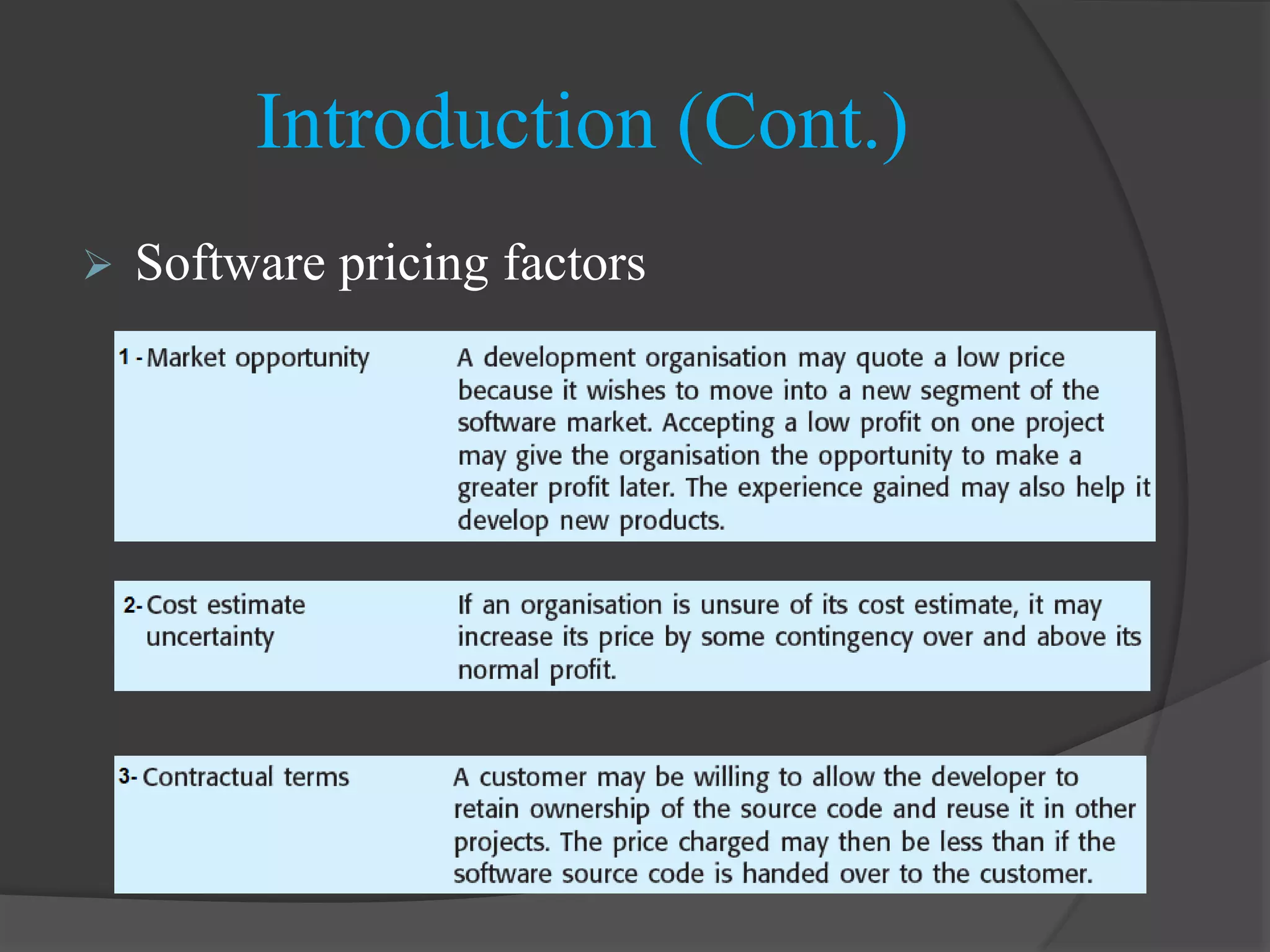
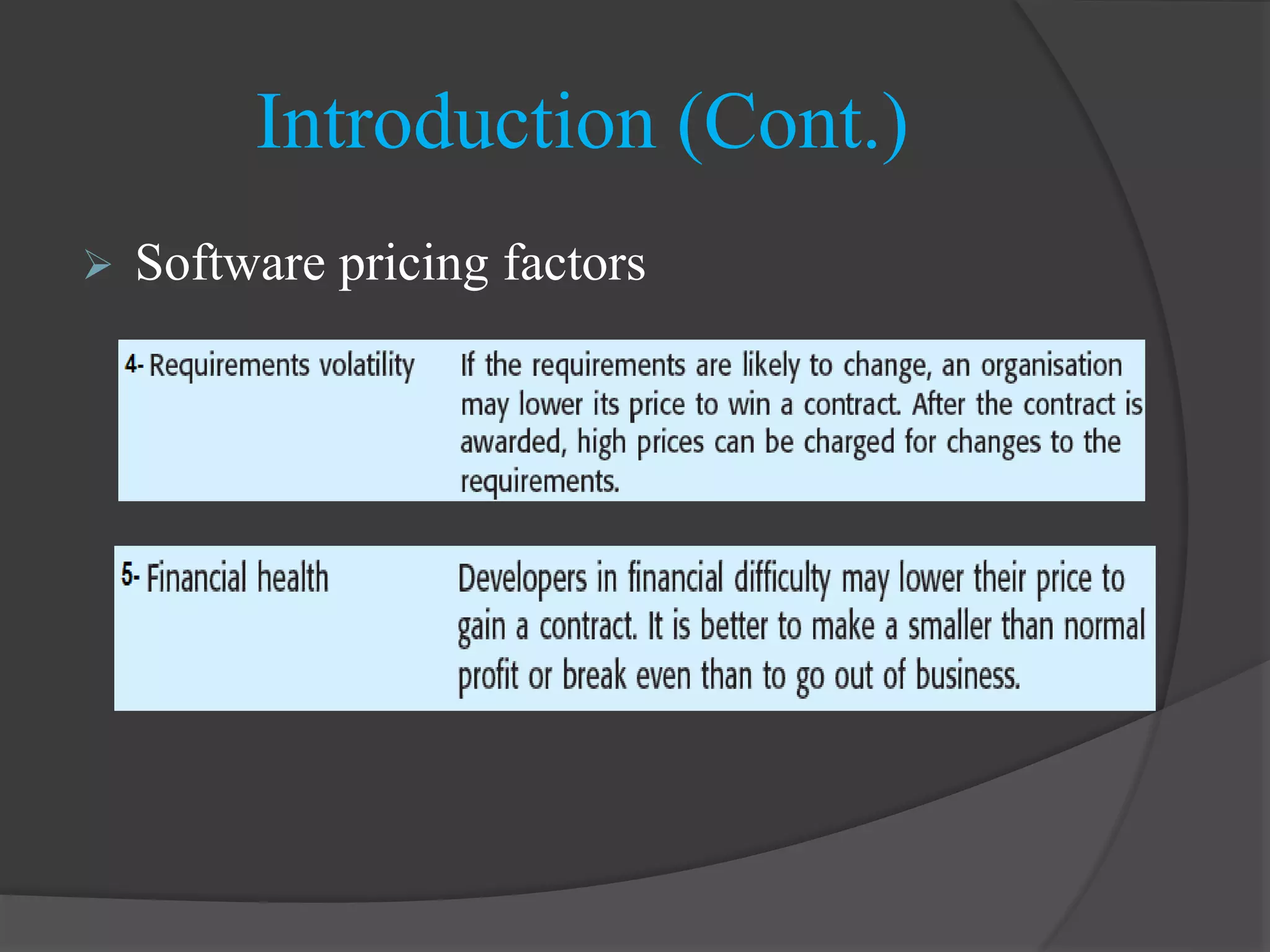
Pricing is influenced by various factors including market opportunity, cost uncertainty, and contractual terms.
Additional factors affecting software pricing are acknowledged but not detailed on this slide.
More factors impacting software pricing are continued but not elaborated here.
Software productivity is measured as output versus input, wanting to quantify functionality produced.
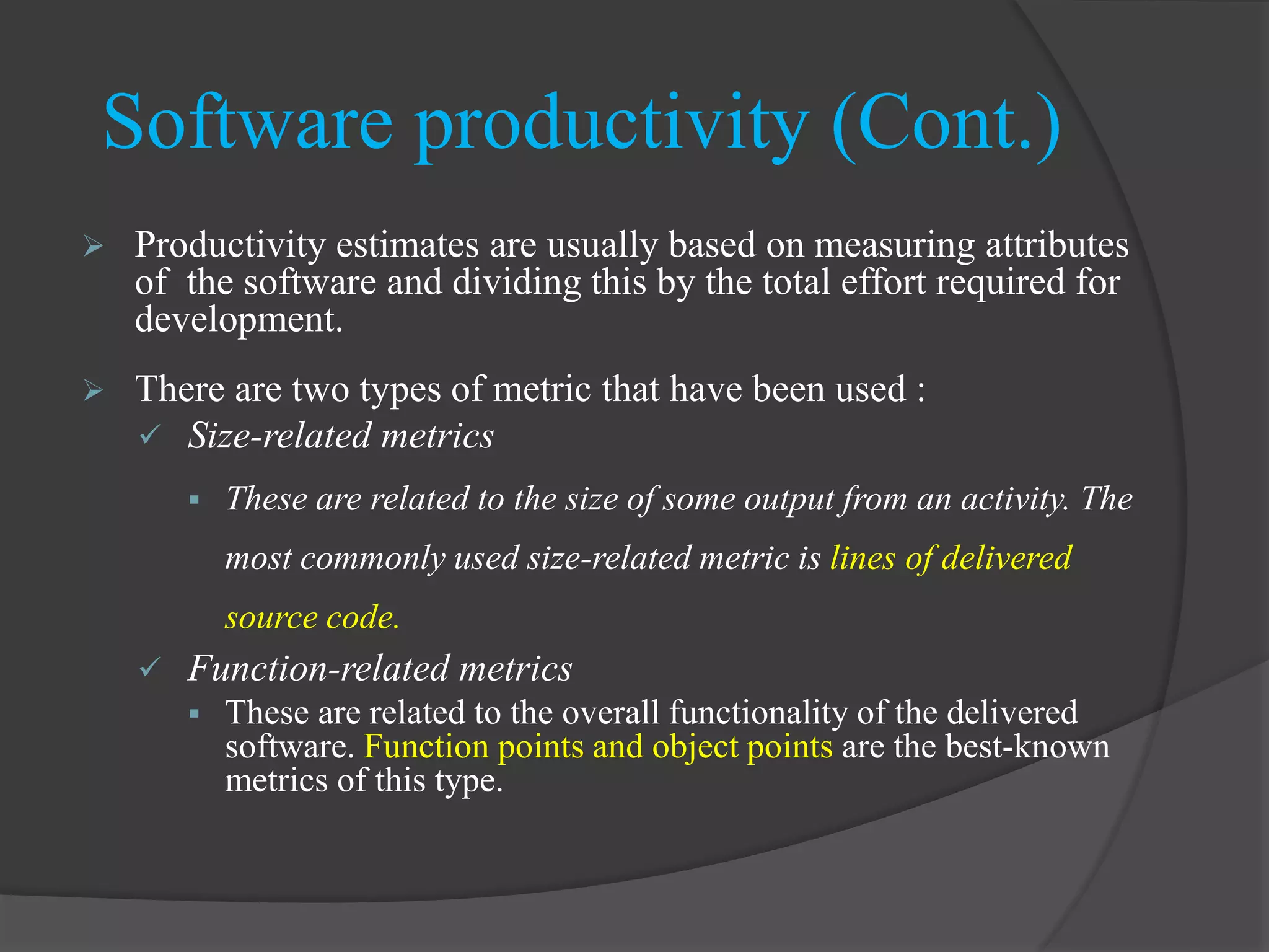
Productivity metrics consist of size-related metrics (like lines of code) and function-related metrics.
LOC/pm metric calculates productivity based on source lines of code delivered per programmer-month.
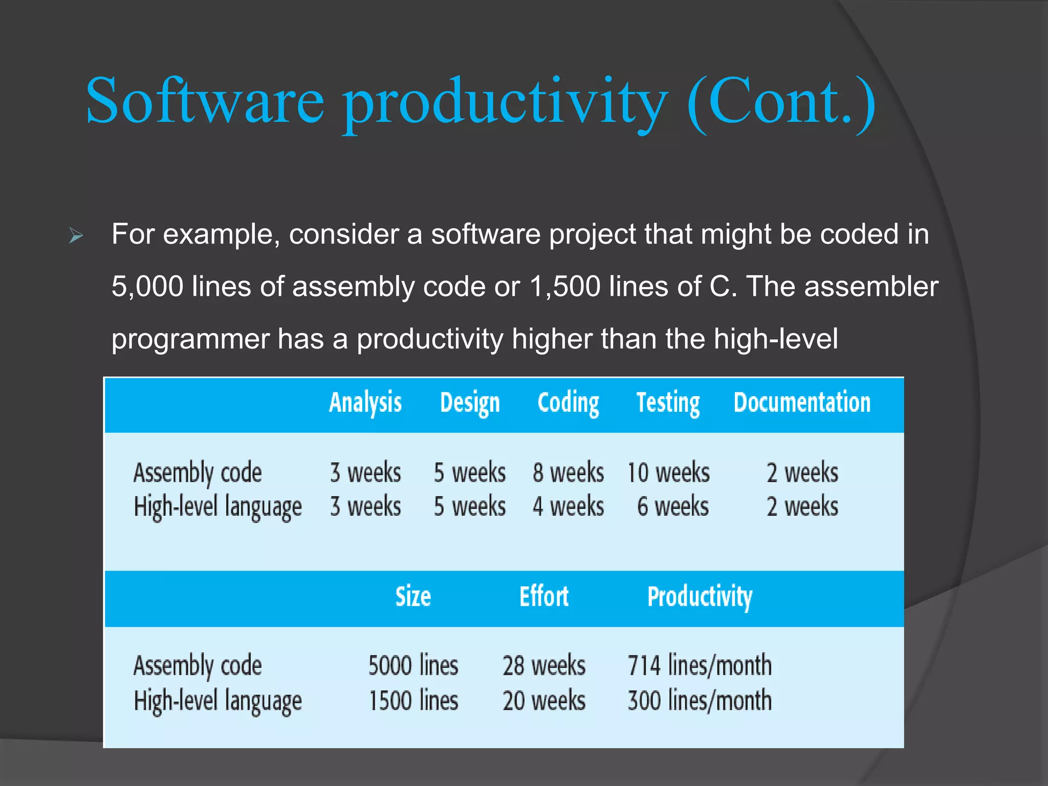
Productivity varies by programming language; lower level languages yield higher LOC productivity.
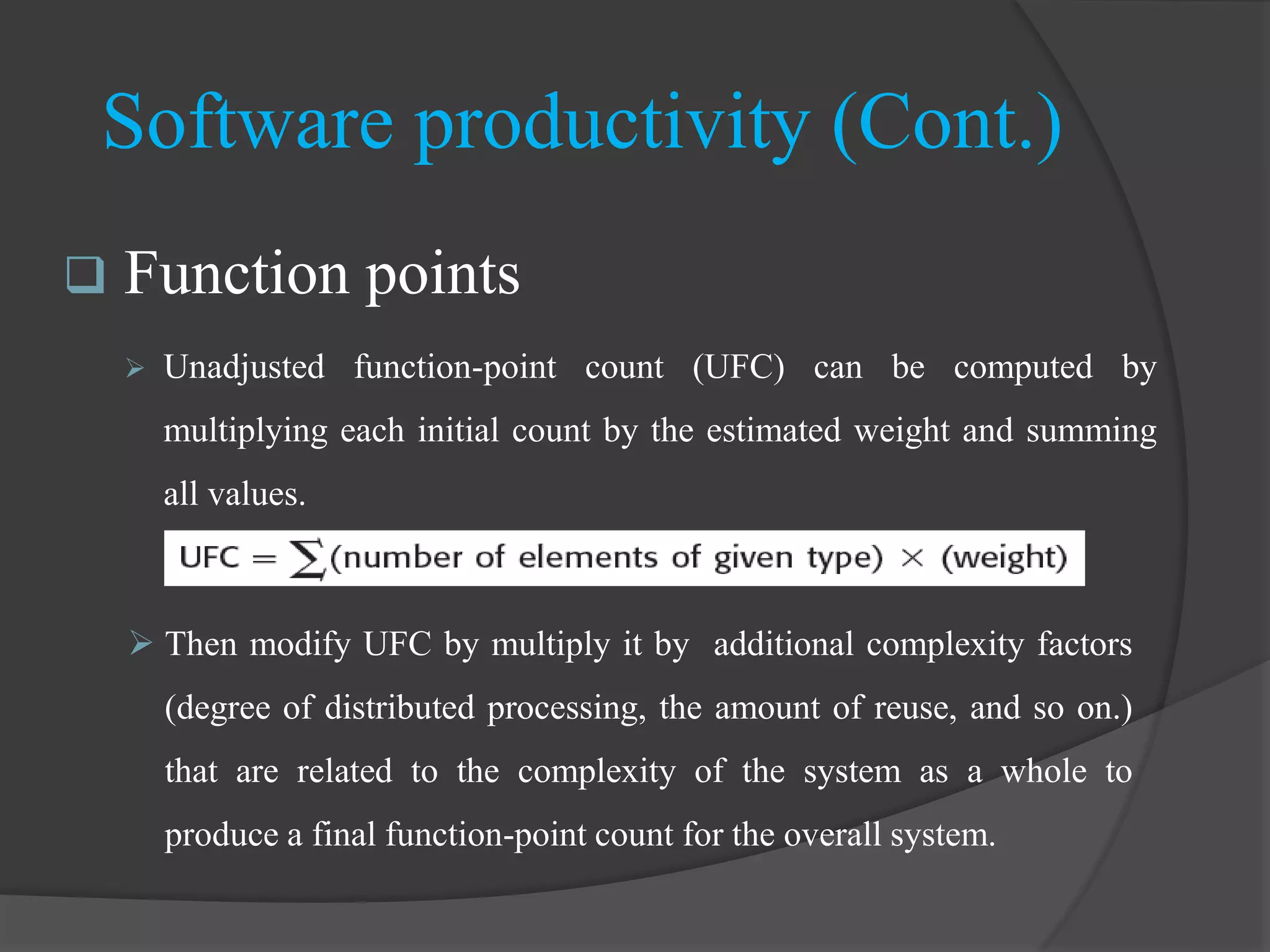
Function points measure productivity by assessing program features, calculated per person-month.
The function-point metric factors in complexity, which affects implementation time and effort.
UFC is calculated by summarizing weighted function-point counts, considering complexity factors.
Function points consider project complexity, unlike size measurement which is susceptible to subjective variability.
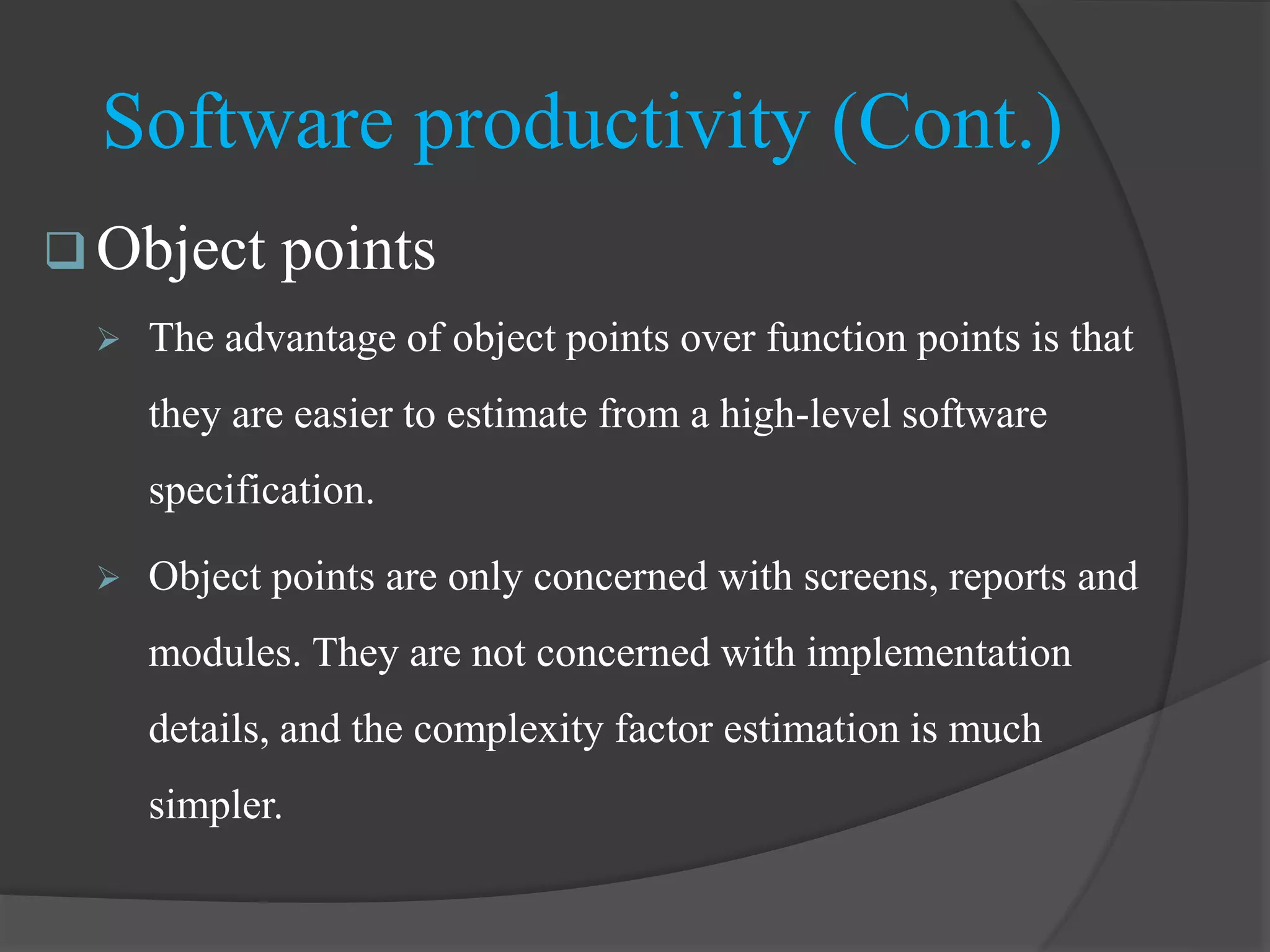
Object points, an alternative metric, measure screens, reports, and modules, simplifying complexity estimation.
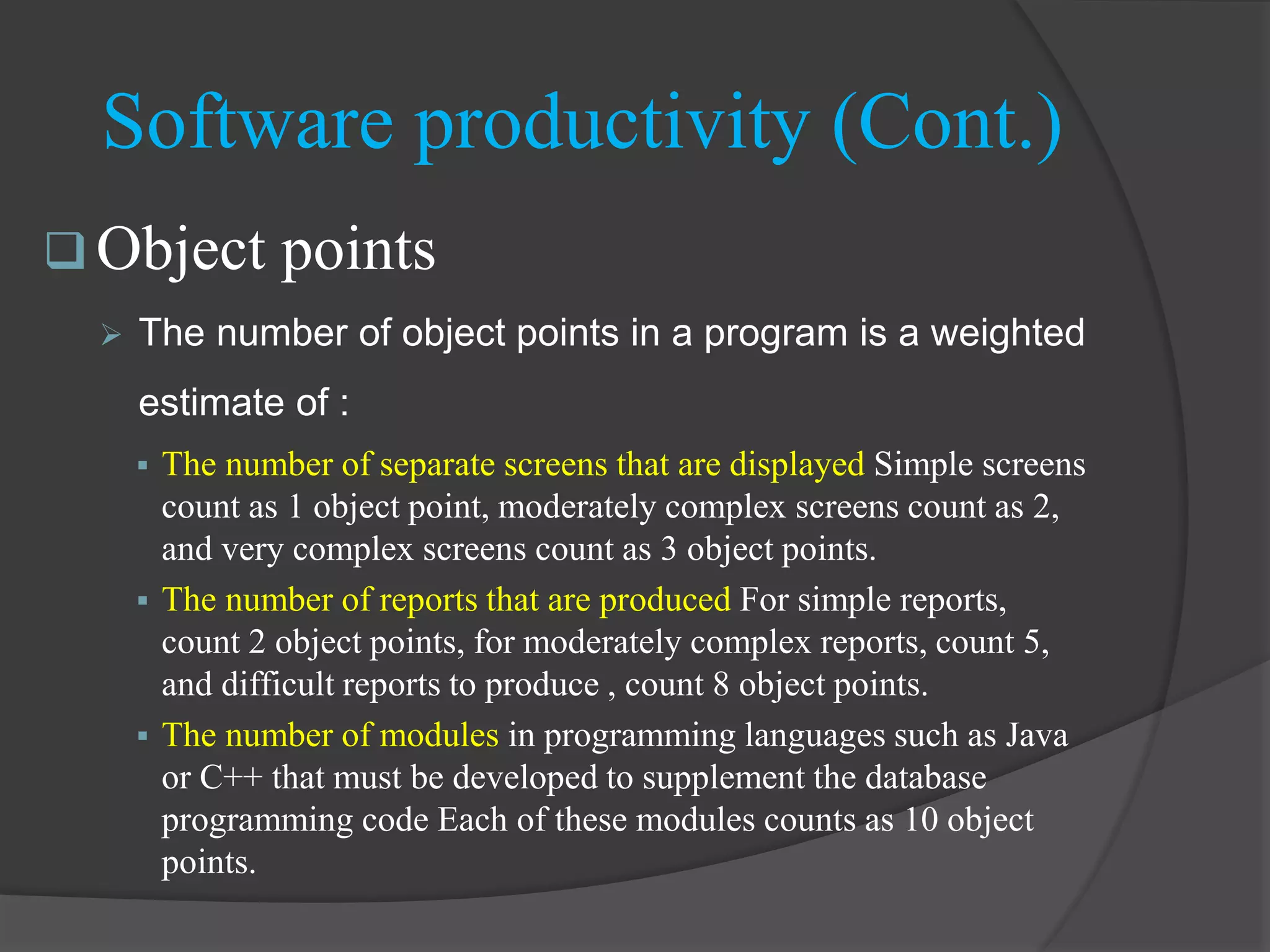
The number of object points is based on the count of screens and reports produced with weighted values.
Object points provide easier estimation compared to function points, focusing on outputs instead of implementation details.
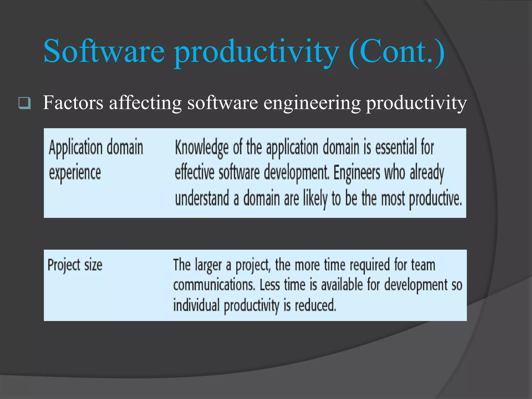
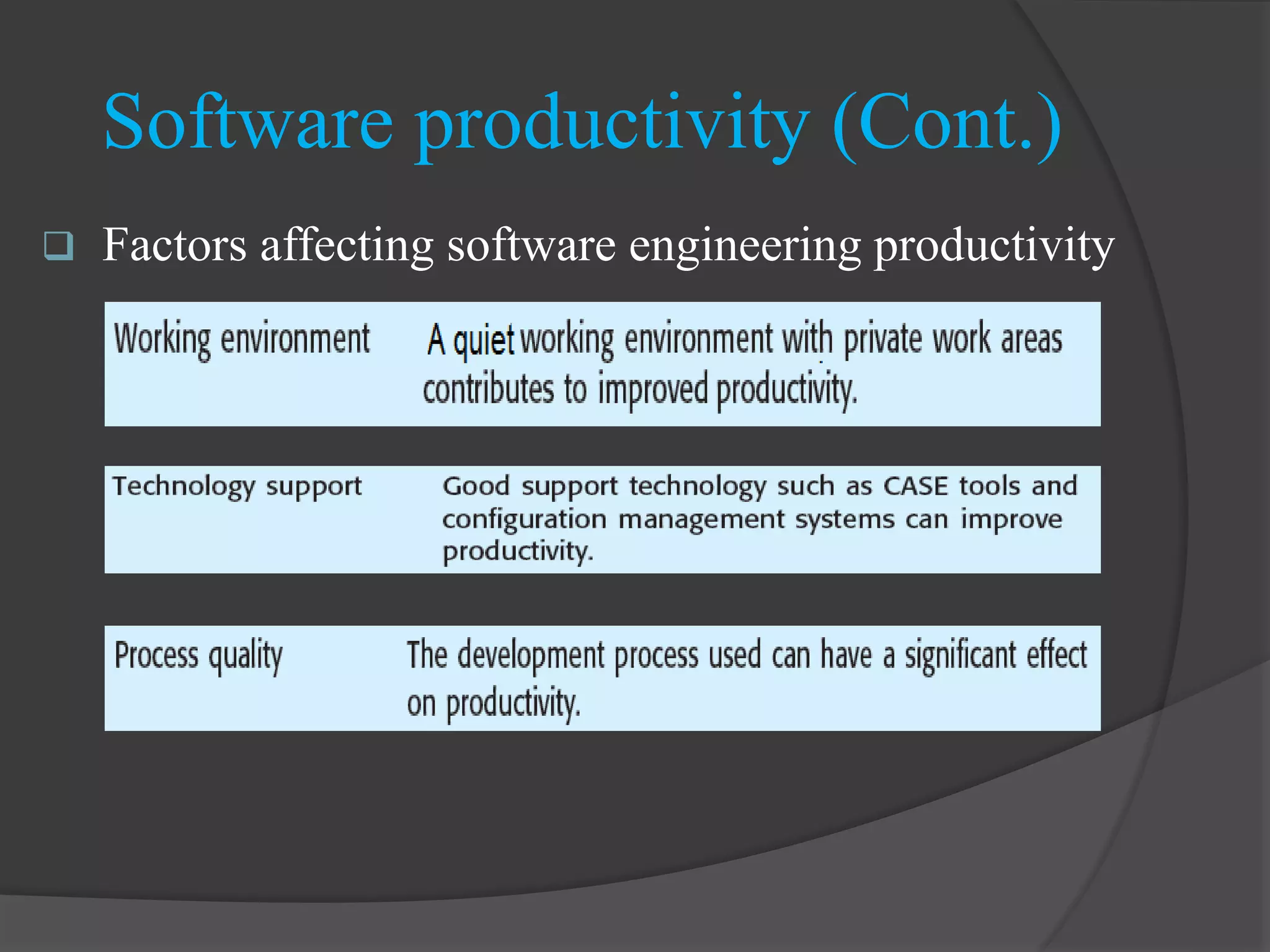
Various factors influencing software engineering productivity are addressed but not detailed.
Further factors affecting productivity are mentioned but not elaborated in this section.
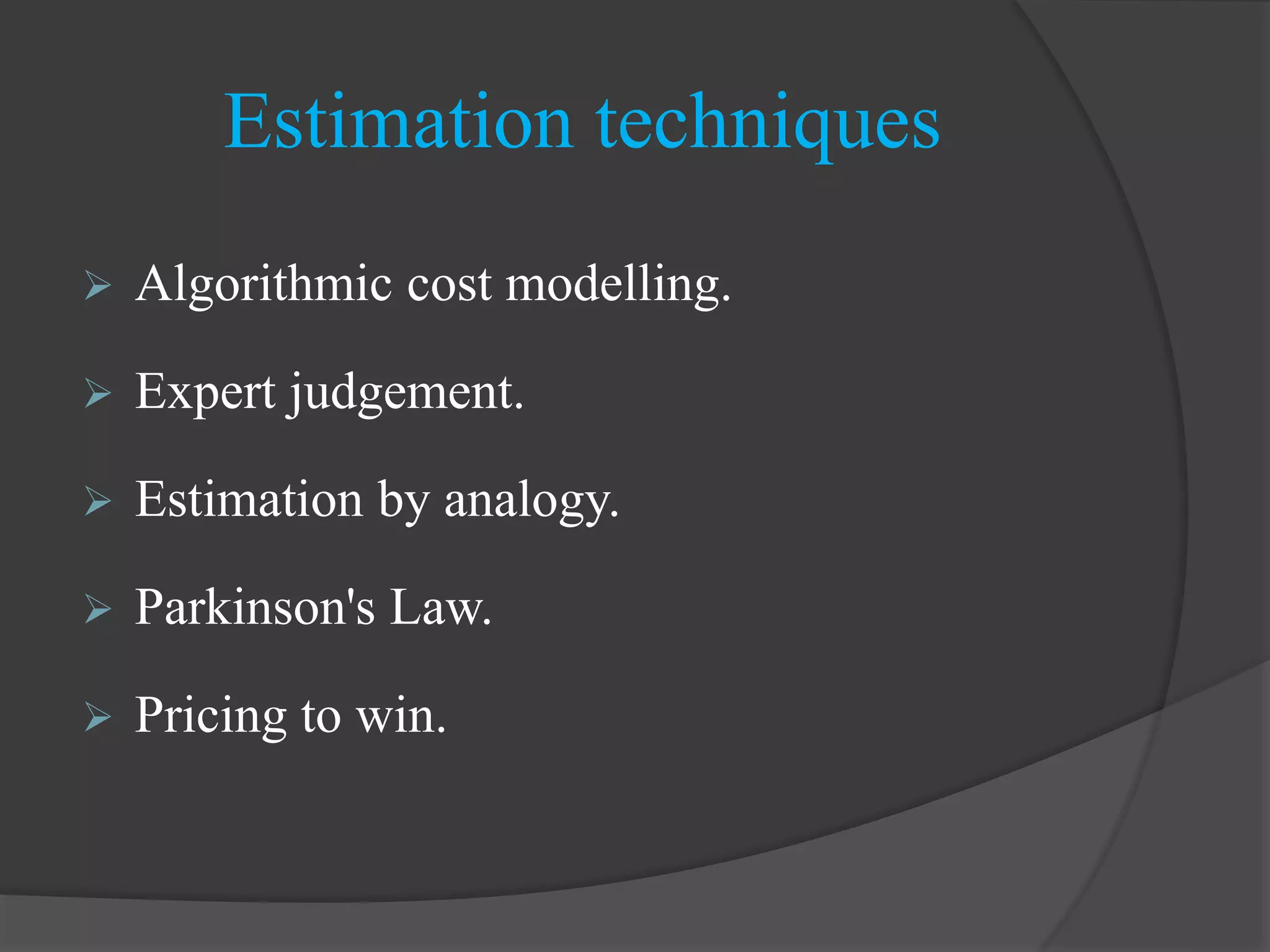
Techniques for estimation include algorithmic modelling, expert judgment, analogy, Parkinson's Law, and pricing tactics.
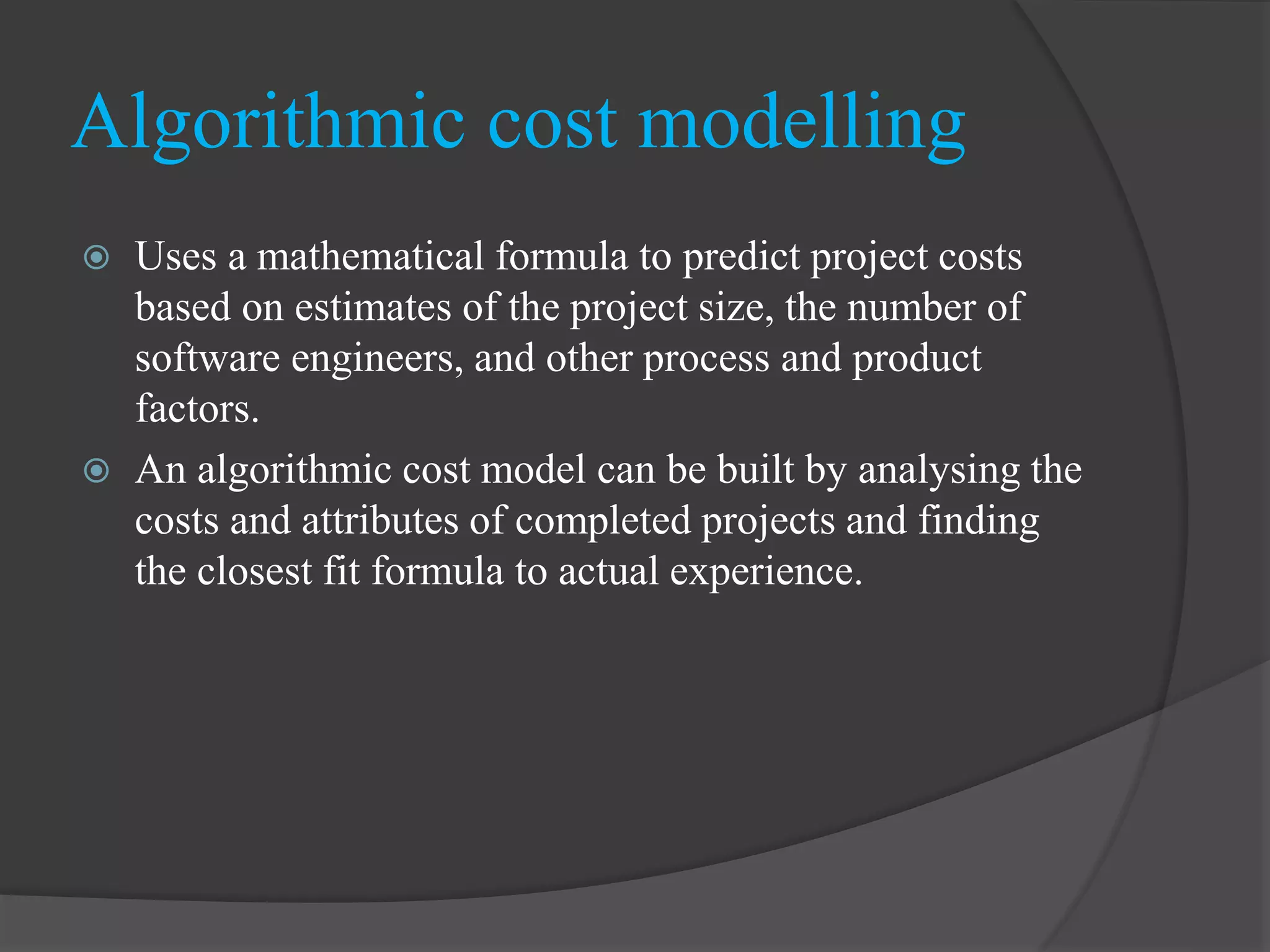
Historical cost data is used in algorithmic models to predict project costs relating metrics to effort.
Experts provide cost estimates that are compared and refined through discussions until a consensus is achieved.
This technique estimates costs by comparing to previously completed projects in the same domain.
Work expands to fit the available time; project costs may thus be driven by resources rather than metrics.
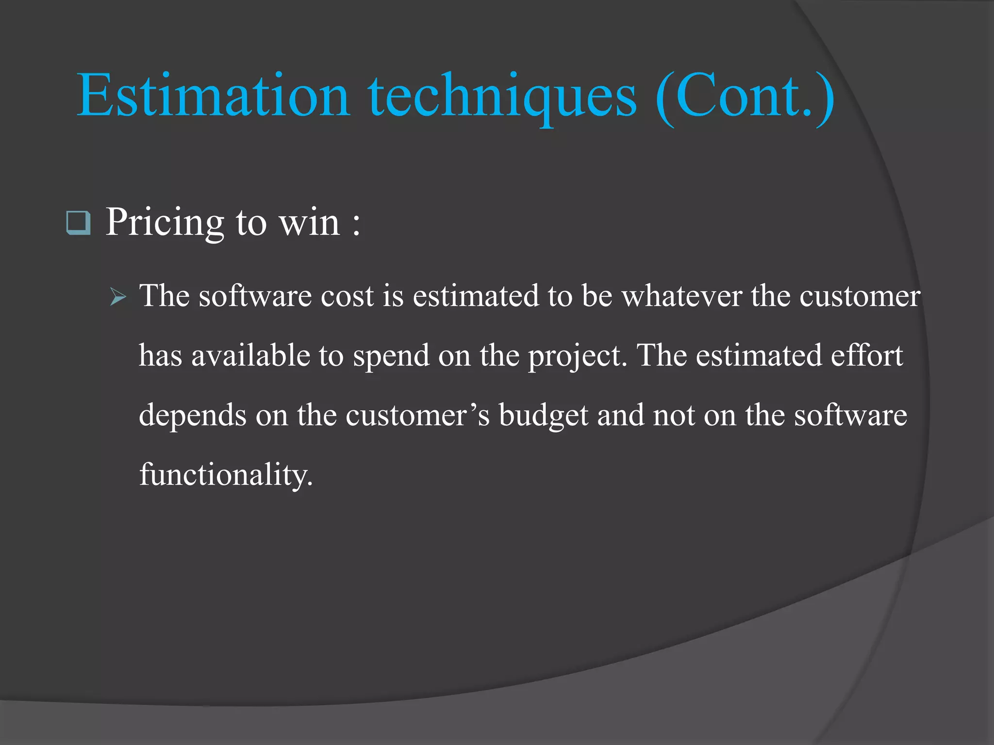
Estimation may hinge on the customer's budget rather than the required software functionality.
Mathematical formulas are used in algorithmic models to predict costs based on various project factors.
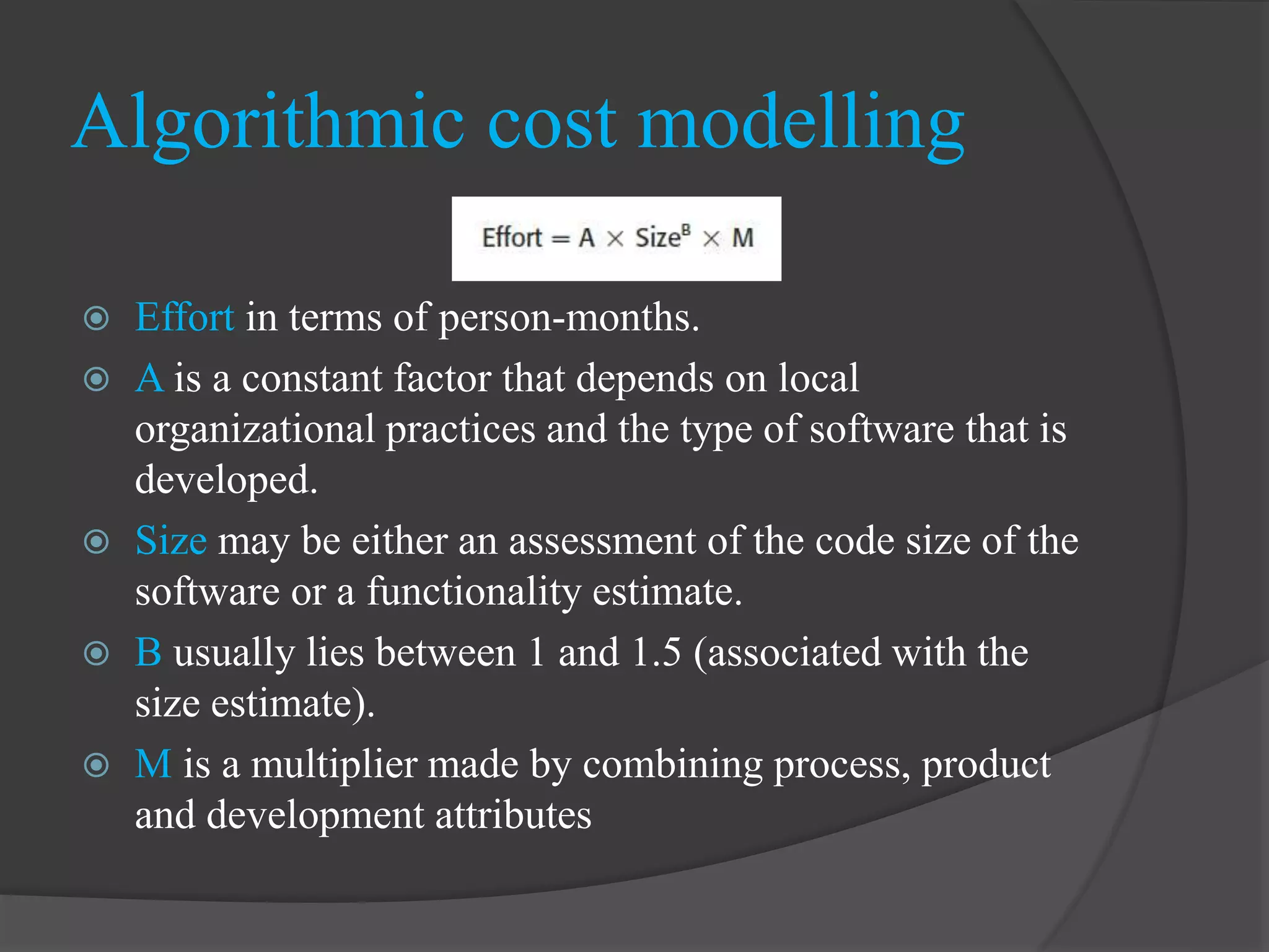
Key constants and variables in algorithmic models, including effort, size, and factors affecting the model.
Estimates in algorithmic models can be hard, particularly for size and subjective factor evaluations.
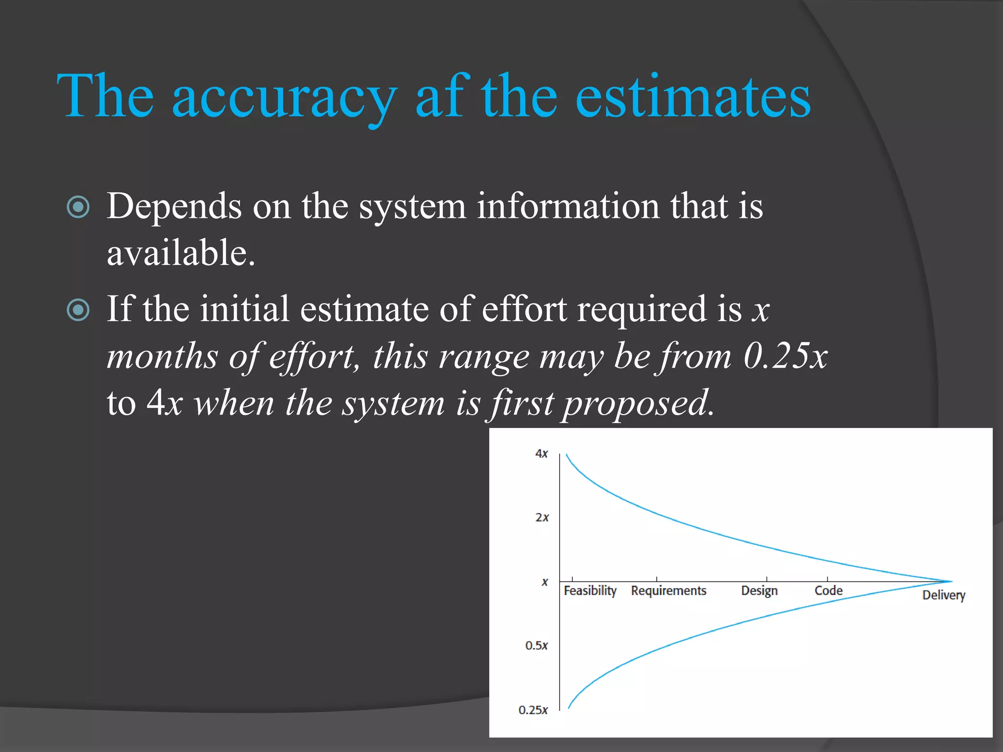
Initial effort estimates can vary widely, indicating significant uncertainty in software project estimations.
COCOMO model uses data from numerous projects to derive formulae that link size and effort for software development.
COCOMO is empirical, well documented, widely used, and incorporates changes in software development since 1981.
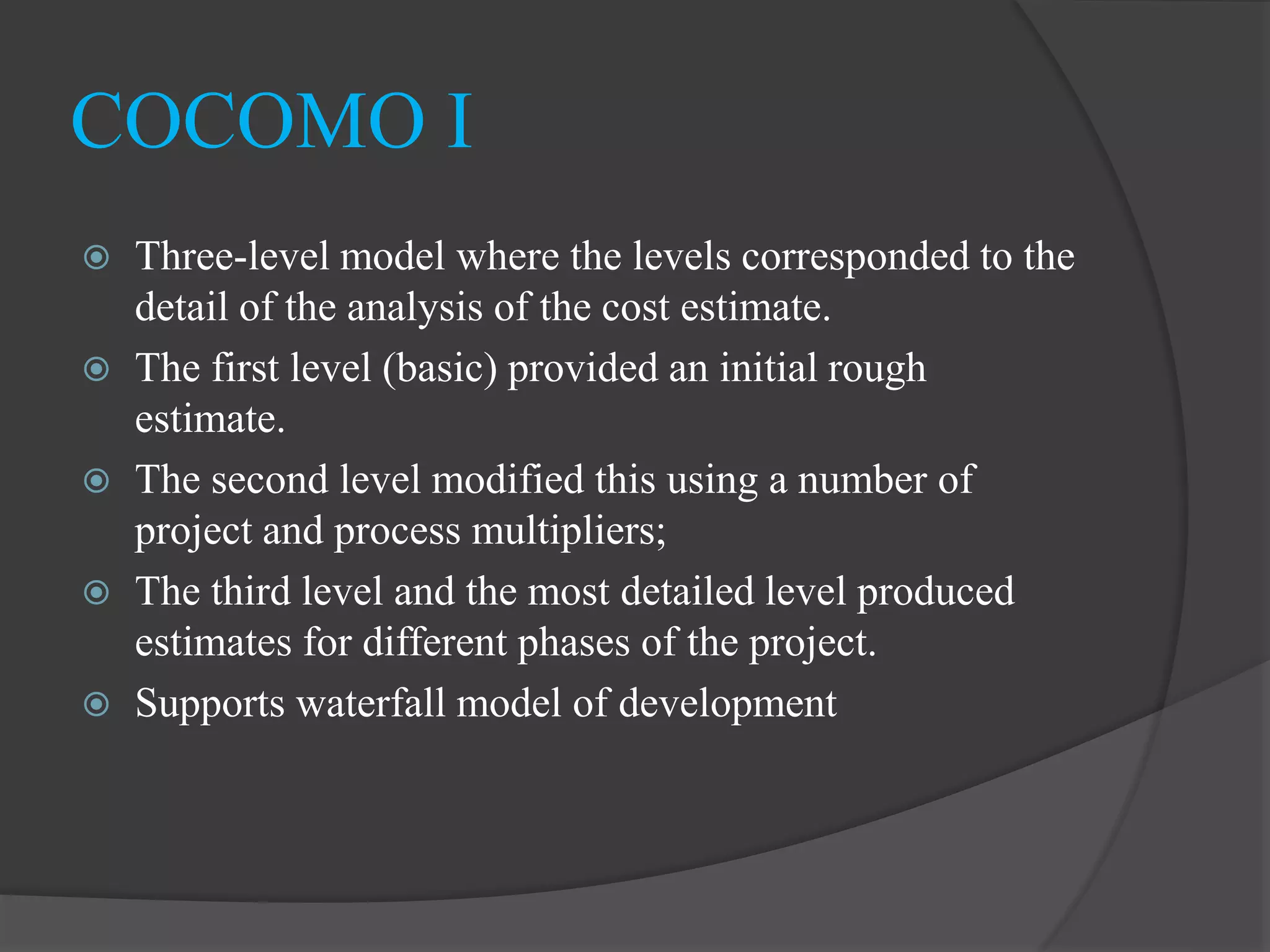
Levels of the COCOMO model provide rough to detailed project estimates, supporting the waterfall development approach.
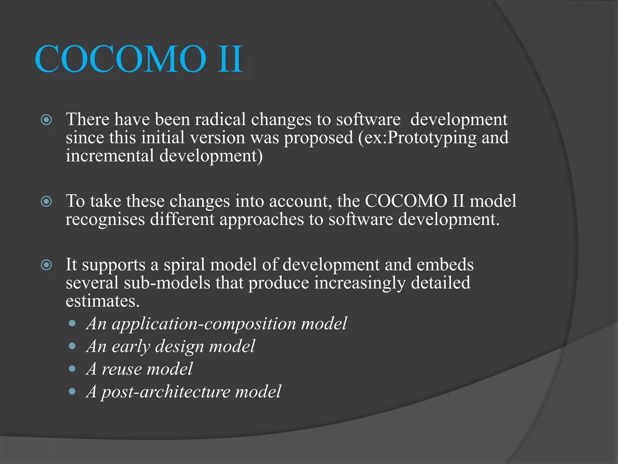
COCOMO II adapts to modern development methods like prototyping and incremental approaches.
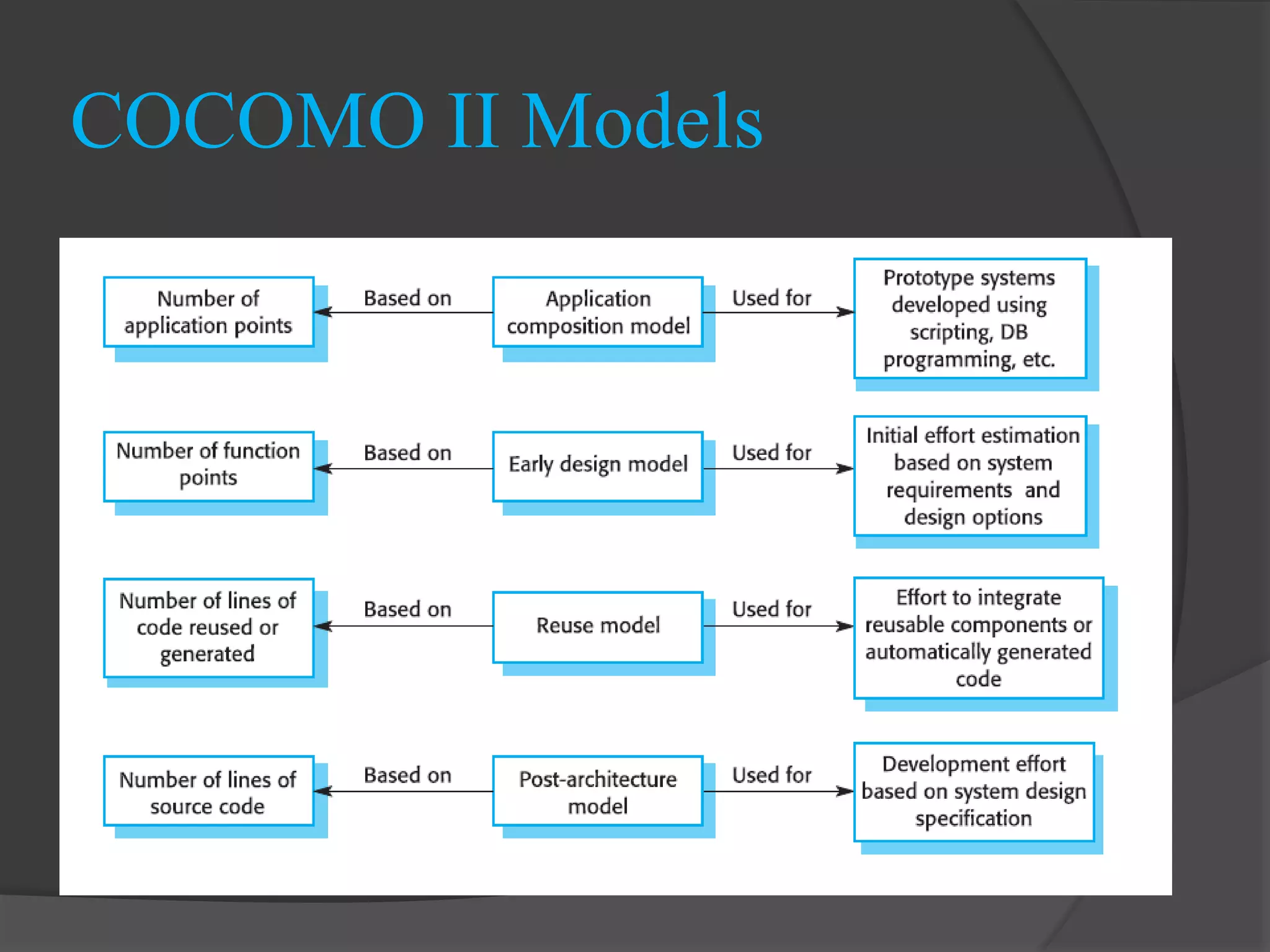
Different sub-models under COCOMO II yield varying estimates based on agile and adaptive methodologies.
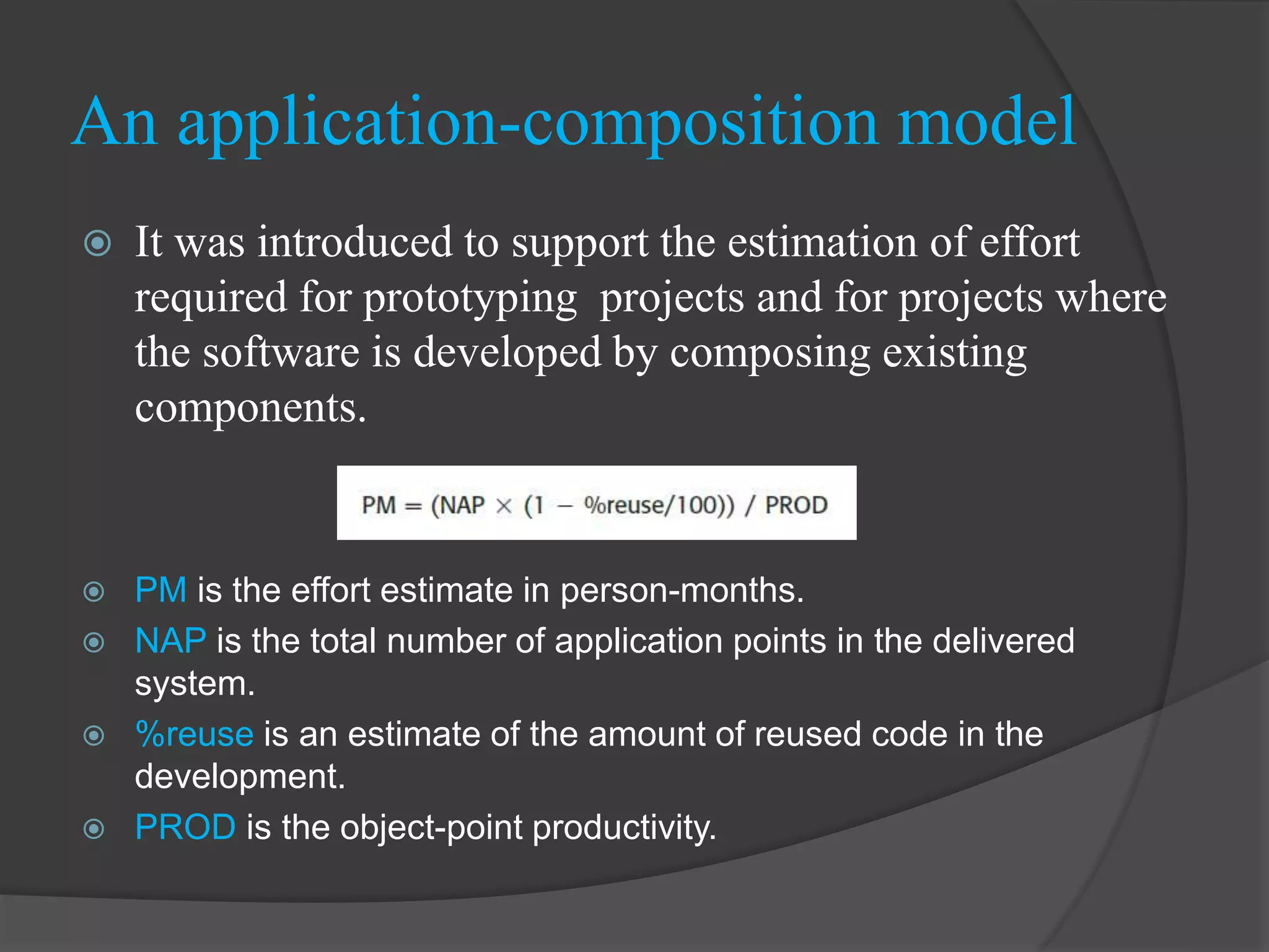
Effects of reuse in software coding are accounted for in effort estimates for application-composition projects.
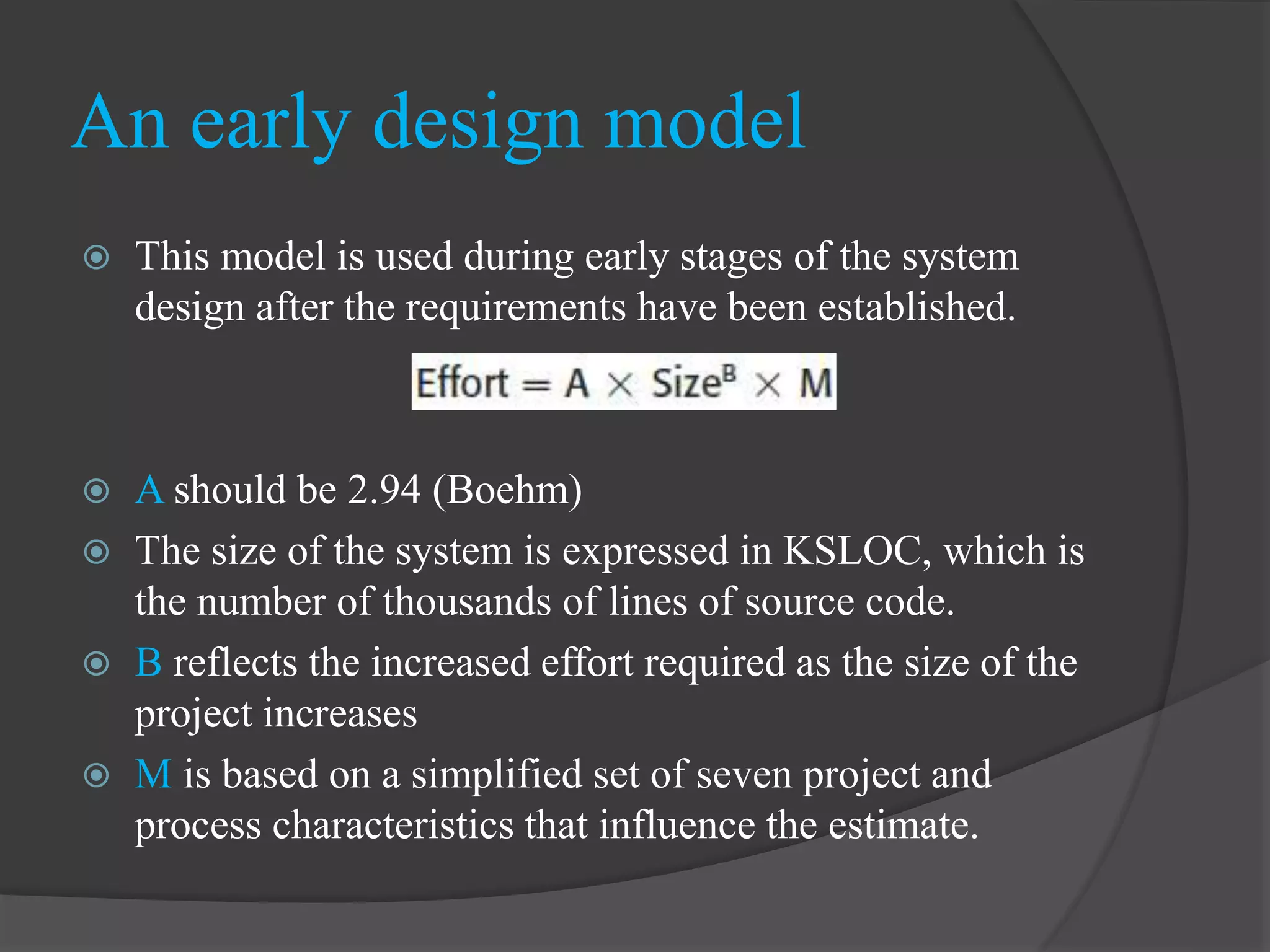
Early design model factors influence estimates based on established requirements after initial architecture.
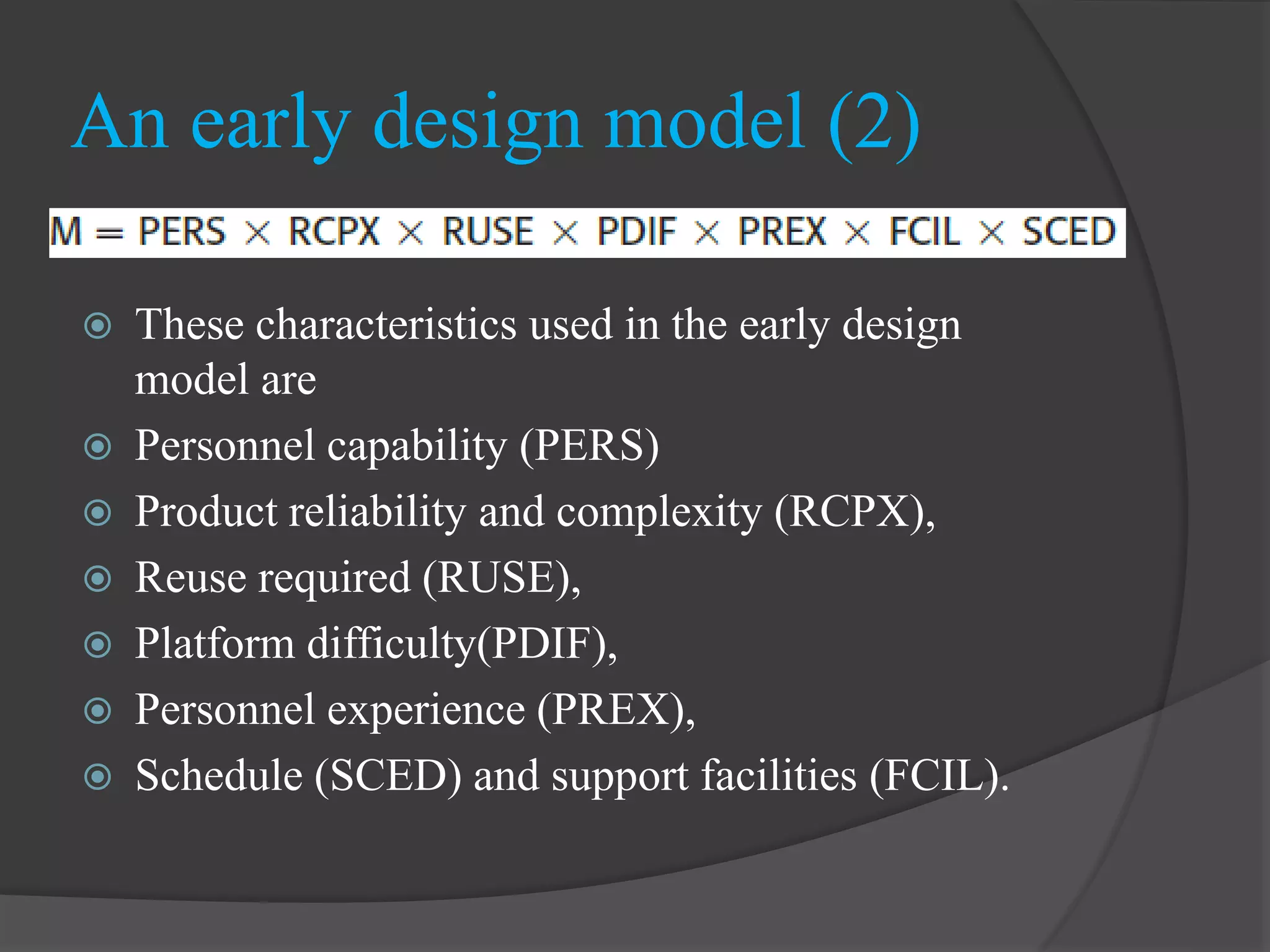
Factors like personnel capability, product reliability, and project complexity influence software cost estimation.
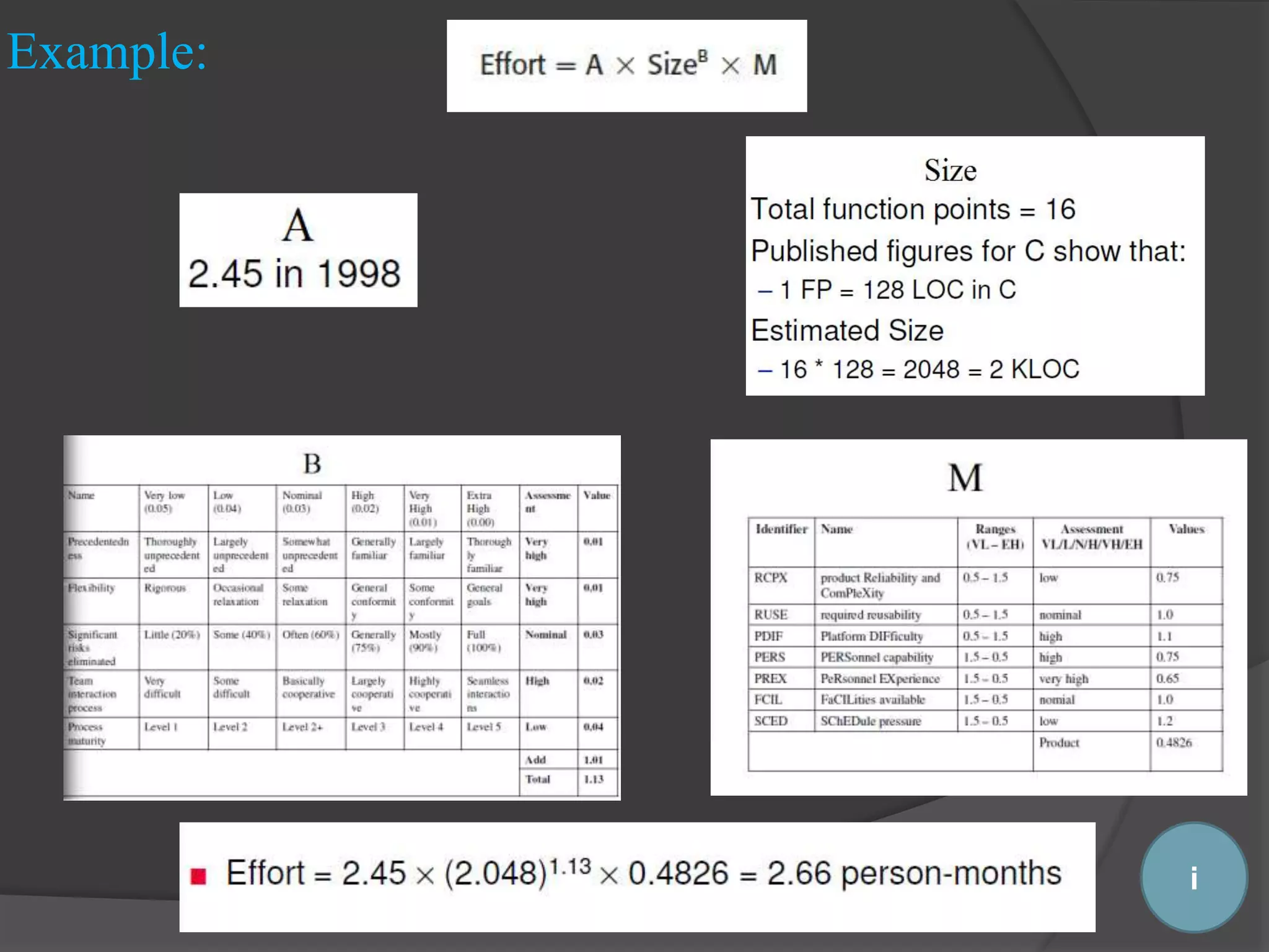
Specific examples of project estimation methodologies applied in software projects are outlined.
Estimates of integration effort for reusable components are calculated based on specific metrics.
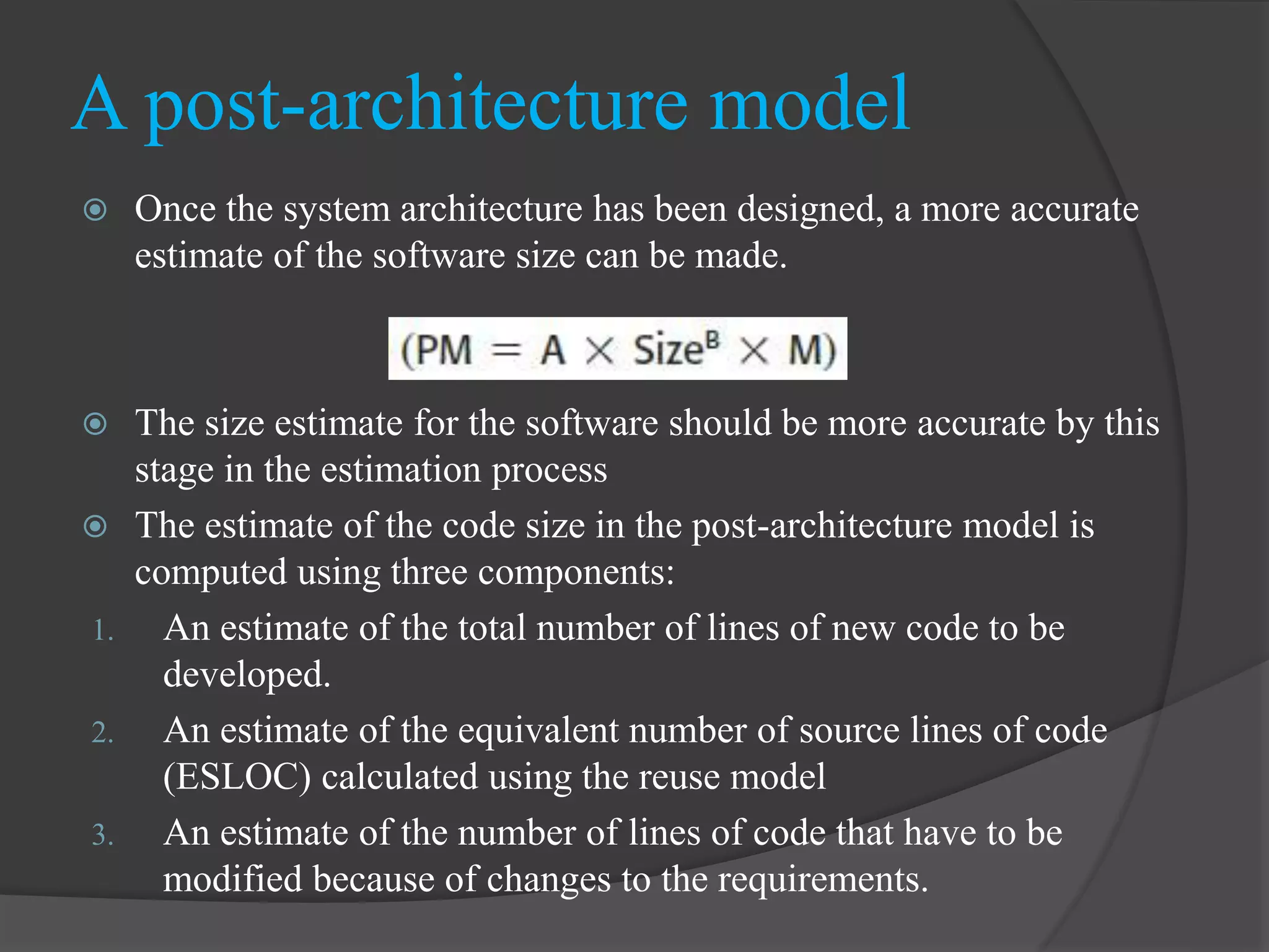
More accurate size estimates post-architecture involve assessing new code, reused code, and modification needs.
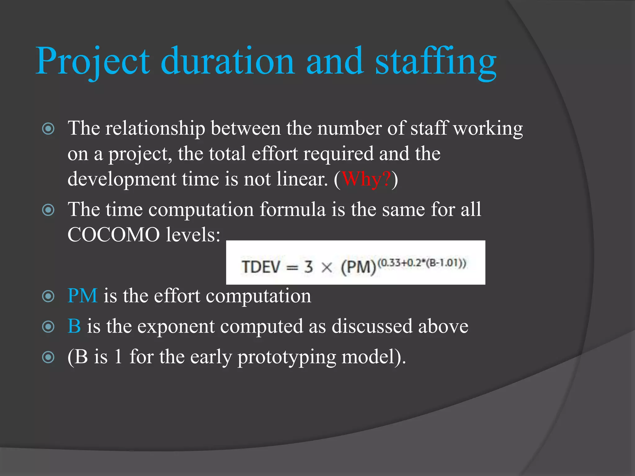
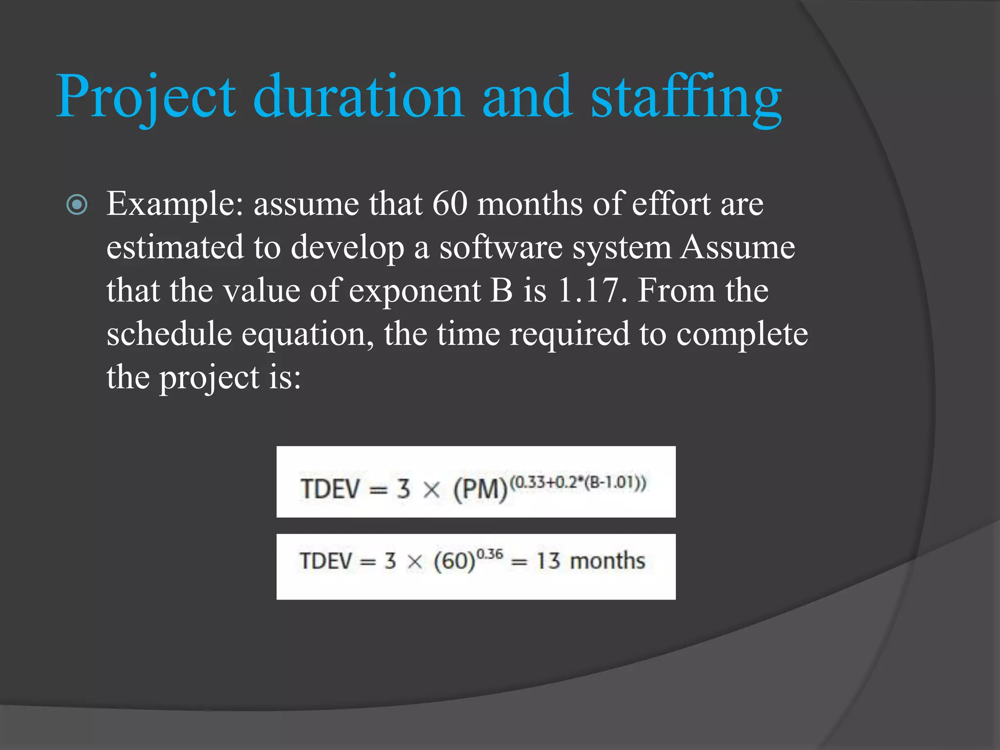
The relationship between staff, effort, and project time is non-linear, requiring careful calculations.
An example illustrates how to estimate project duration based on total effort and exponent calculation.
These techniques leverage past knowledge for better cost estimation in new software development projects.
Efforts are estimated using fuzzy functions to provide flexibility in cost predictions based on uncertainty.
These algorithms are applied to enhance estimation accuracy in the COCOMO model compared to standard approaches.
BBNs model probabilistic relationships in uncertain situations, facilitating improved software product estimates.
A list of references used throughout the presentation, covering various topics in software cost estimation.