SPM-UNIT - V
SOFTWARE RELIABILITY
Prof. Kanchana Devi
Software Reliability
Prof. Kanchana Devi
2
 Categorising and specifying the reliability
of software systems
 Informal Definition:
 Reliability is a measure of how well system users
think it provides the services they require.
 Probability of a software component will
produce an incorrect output
 Software can continue to operate after a bad
result
………
Prof. Kanchana Devi
3
 Software Reliability is the probability of failure-
free software operation for a specified period
of time in a specified environment.
 Software Reliability is also an important factor
affecting system reliability.
 It differs from hardware reliability in that it
reflects the “design perfection”, rather than
manufacturing perfection.
 The high complexity of software is the major
contributing factor of Software Reliability
problems.
Traditional Methods For Improving
Software Reliability
Prof. Kanchana Devi
4
 Three main techniques are used in industrial and
open source projects to improve software reliability:
 Manual Testing
 Code Reviews:
 Modifications are reviewed by experienced developers
before being committed to the code base.
 Coding Standards:
 Requiring that all developers adhere to a set of rules when
writing or maintaining code.
 Coding standards can improve source code readability,
making it easier to spot defects, and
 Ban the use of programming idioms that are arguably
dangerous.
Reliability Problems
Prof. Kanchana Devi
5
 They depend fundamentally on human
reasoning and judgments
 They do not provide guarantees
Measuring Reliability
Prof. Kanchana Devi
6
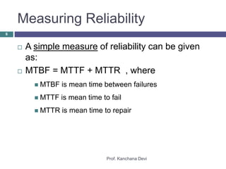
 A simple measure of reliability can be given
as:
 MTBF = MTTF + MTTR , where
 MTBF is mean time between failures
 MTTF is mean time to fail
 MTTR is mean time to repair
Software Reliability Models
Prof. Kanchana Devi
7
 Error Seeding
 Reliability growth
 Non-Homogeneous Poisson process (NHPP)
Error Seeding
Prof. Kanchana Devi
8
 Estimates the number of errors in a program.
 Errors are divided into
 Indigenous Errors
 Induced (seeded) Errors.
 The unknown number of indigenous errors is
estimated from the number of induced errors.
 The ratio of the two types of errors obtained
from the testing data.
Reliability Growth
9
 Measures and predicts the improvement of
reliability through the testing process using a
growth function to represent the process.
 Growth Function has two types of variables:
 Independent Variables
 Dependent Variables
 Independent Variables of the growth function
could be time and number of test cases (or
testing stages)
 Dependent Variables can be reliability, failure
rate or cumulative number of errors detected.
Non-homogeneous Poisson process (NHPP)
Prof. Kanchana Devi
10
 Provide an analytical framework for describing
the software failure phenomenon during
testing.
 The main issue is to estimate the mean value
function of the cumulative number of failures.
Prof. Kanchana Devi
11
)
],[infailuresofNumber
()(





 f
 A typical measure (failures per unit time) is the
failure intensity (rate) given as:
 where  = program CPU time (in a time shared
computer) or wall clock time (in an
embedded system).
Issues in SR:
Prof. Kanchana Devi
12
 SR Growth models are generally “black box”
- no easy way to account for a change in
the “operational profile”
 “Operational profile”: description of the input
events expected to occur in actual software
operation – how it will be used in practice
Prof. Kanchana Devi
13
 Many models have been proposed, perhaps
the most prominent are:
 Musa Basic model
 Musa/Okomoto Logarithmic model
 Some models work better than others
depending on the application area and
operating characteristics:
 i.e. interactive?
 data intensive?
 control intensive?
 real-time?
Choice of Model - Basic Model:
Prof. Kanchana Devi
14
 For studies or predictions before execution
and failure data available
 Using study of faults to determine effects of a
new software engineering technology
 The program size is changing continually or
substantially (i.e. during integration)
Logarithmic Model
Prof. Kanchana Devi
15
 System subjected to highly non-uniform
operational profiles.
 Highly predictive validity is needed early in the
execution period.
 The rapidly changing slope of the failure
intensity during early stages can be better
fitted with the Logarithmic Poisson than the
basic model .

Spm unit v-software reliability-

  • 1.
    SPM-UNIT - V SOFTWARERELIABILITY Prof. Kanchana Devi
  • 2.
    Software Reliability Prof. KanchanaDevi 2  Categorising and specifying the reliability of software systems  Informal Definition:  Reliability is a measure of how well system users think it provides the services they require.  Probability of a software component will produce an incorrect output  Software can continue to operate after a bad result
  • 3.
    ……… Prof. Kanchana Devi 3 Software Reliability is the probability of failure- free software operation for a specified period of time in a specified environment.  Software Reliability is also an important factor affecting system reliability.  It differs from hardware reliability in that it reflects the “design perfection”, rather than manufacturing perfection.  The high complexity of software is the major contributing factor of Software Reliability problems.
  • 4.
    Traditional Methods ForImproving Software Reliability Prof. Kanchana Devi 4  Three main techniques are used in industrial and open source projects to improve software reliability:  Manual Testing  Code Reviews:  Modifications are reviewed by experienced developers before being committed to the code base.  Coding Standards:  Requiring that all developers adhere to a set of rules when writing or maintaining code.  Coding standards can improve source code readability, making it easier to spot defects, and  Ban the use of programming idioms that are arguably dangerous.
  • 5.
    Reliability Problems Prof. KanchanaDevi 5  They depend fundamentally on human reasoning and judgments  They do not provide guarantees
  • 6.
    Measuring Reliability Prof. KanchanaDevi 6  A simple measure of reliability can be given as:  MTBF = MTTF + MTTR , where  MTBF is mean time between failures  MTTF is mean time to fail  MTTR is mean time to repair
  • 7.
    Software Reliability Models Prof.Kanchana Devi 7  Error Seeding  Reliability growth  Non-Homogeneous Poisson process (NHPP)
  • 8.
    Error Seeding Prof. KanchanaDevi 8  Estimates the number of errors in a program.  Errors are divided into  Indigenous Errors  Induced (seeded) Errors.  The unknown number of indigenous errors is estimated from the number of induced errors.  The ratio of the two types of errors obtained from the testing data.
  • 9.
    Reliability Growth 9  Measuresand predicts the improvement of reliability through the testing process using a growth function to represent the process.  Growth Function has two types of variables:  Independent Variables  Dependent Variables  Independent Variables of the growth function could be time and number of test cases (or testing stages)  Dependent Variables can be reliability, failure rate or cumulative number of errors detected.
  • 10.
    Non-homogeneous Poisson process(NHPP) Prof. Kanchana Devi 10  Provide an analytical framework for describing the software failure phenomenon during testing.  The main issue is to estimate the mean value function of the cumulative number of failures.
  • 11.
    Prof. Kanchana Devi 11 ) ],[infailuresofNumber ()(      f  A typical measure (failures per unit time) is the failure intensity (rate) given as:  where  = program CPU time (in a time shared computer) or wall clock time (in an embedded system).
  • 12.
    Issues in SR: Prof.Kanchana Devi 12  SR Growth models are generally “black box” - no easy way to account for a change in the “operational profile”  “Operational profile”: description of the input events expected to occur in actual software operation – how it will be used in practice
  • 13.
    Prof. Kanchana Devi 13 Many models have been proposed, perhaps the most prominent are:  Musa Basic model  Musa/Okomoto Logarithmic model  Some models work better than others depending on the application area and operating characteristics:  i.e. interactive?  data intensive?  control intensive?  real-time?
  • 14.
    Choice of Model- Basic Model: Prof. Kanchana Devi 14  For studies or predictions before execution and failure data available  Using study of faults to determine effects of a new software engineering technology  The program size is changing continually or substantially (i.e. during integration)
  • 15.
    Logarithmic Model Prof. KanchanaDevi 15  System subjected to highly non-uniform operational profiles.  Highly predictive validity is needed early in the execution period.  The rapidly changing slope of the failure intensity during early stages can be better fitted with the Logarithmic Poisson than the basic model .