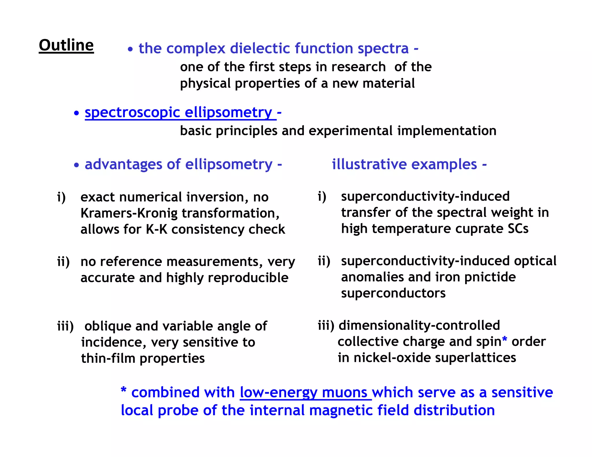
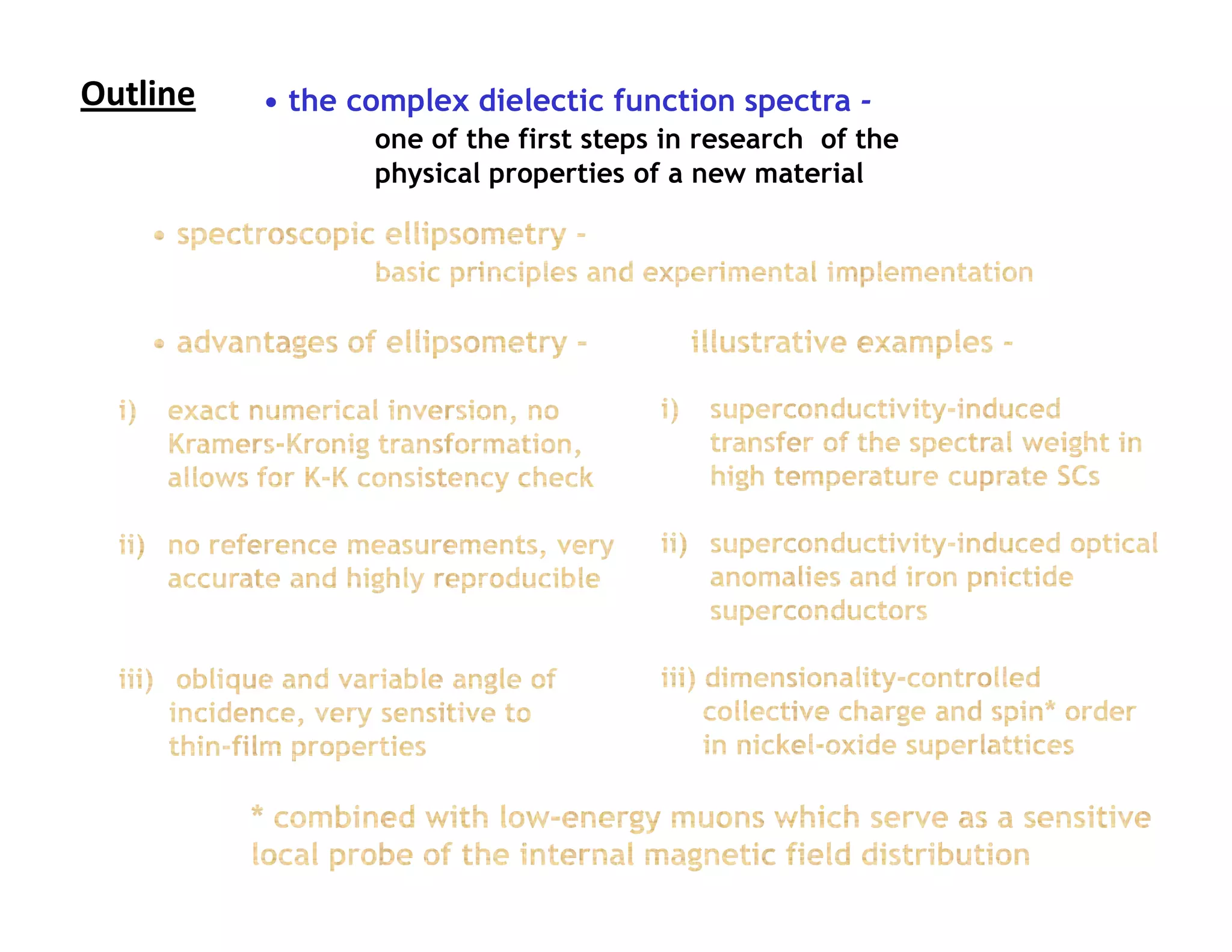
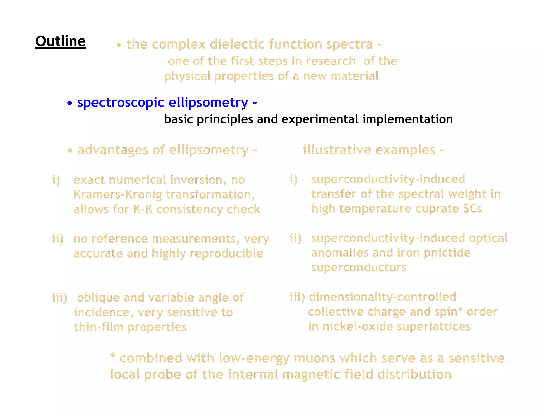
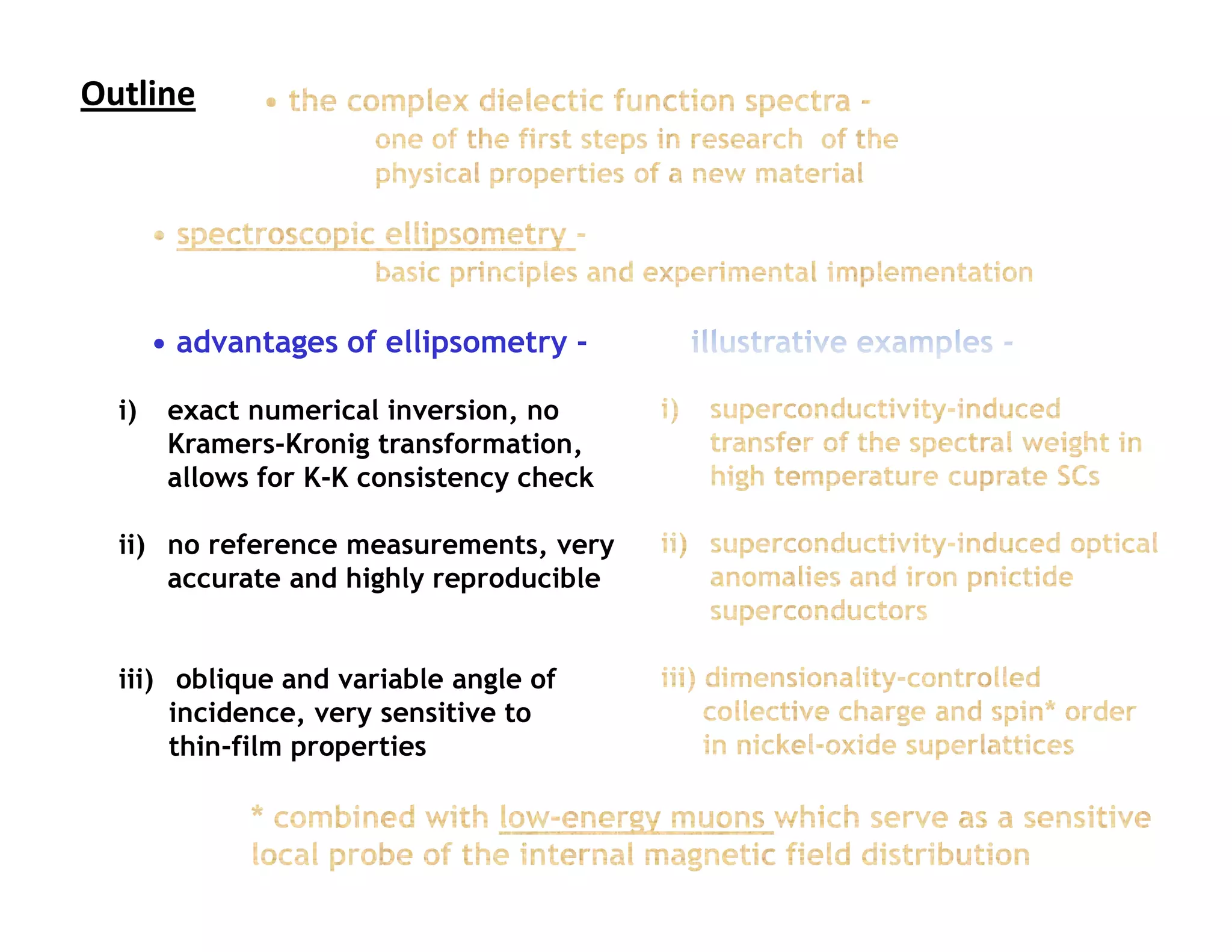
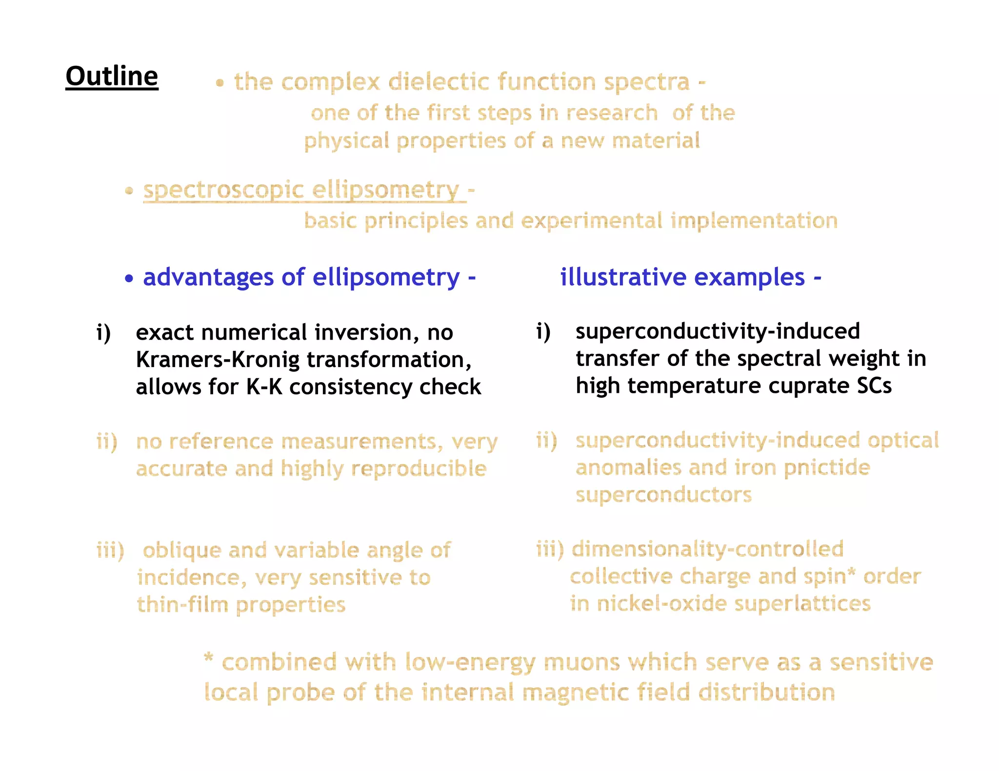
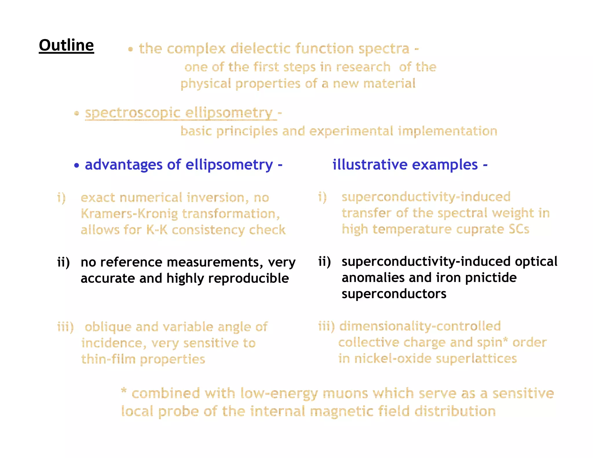
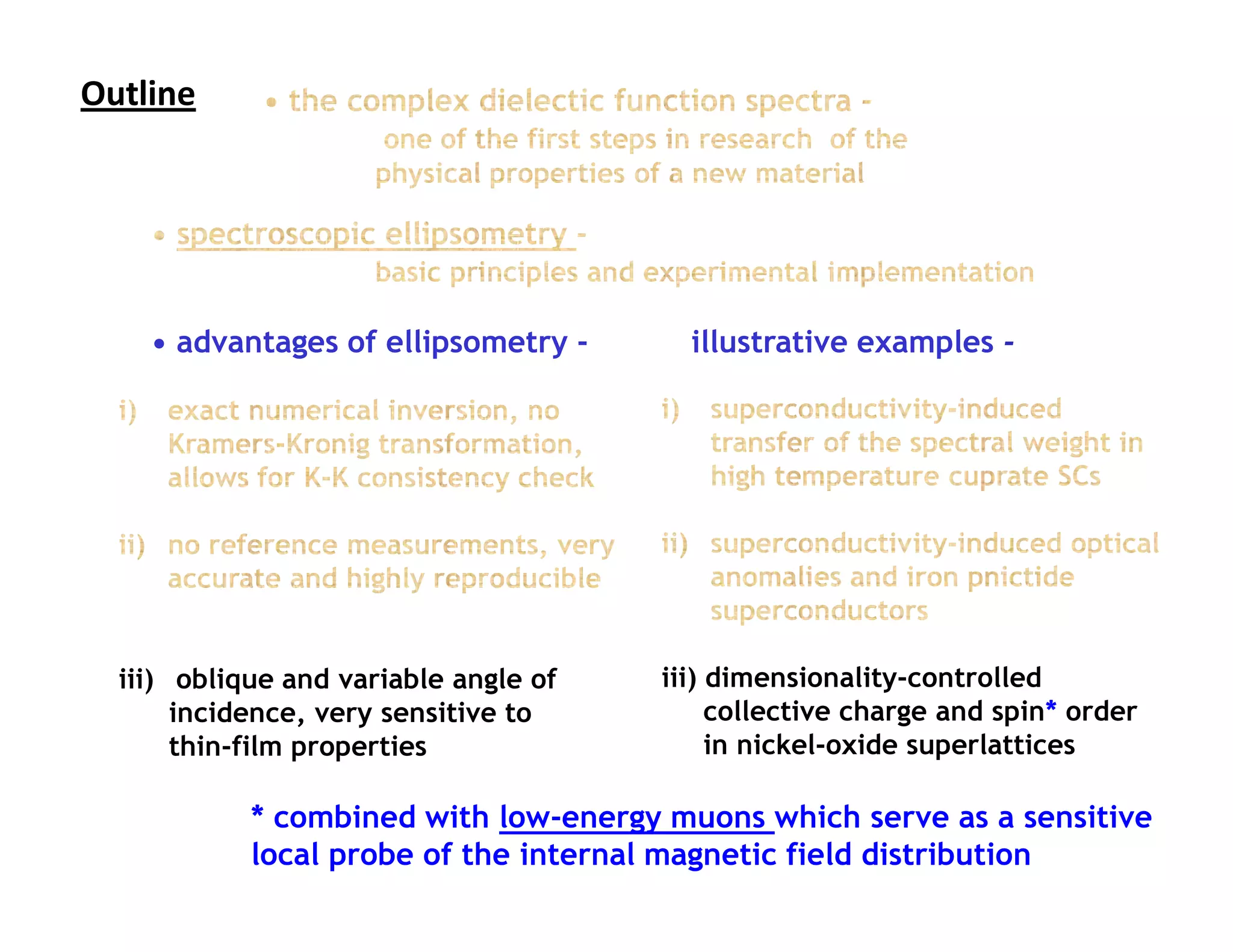
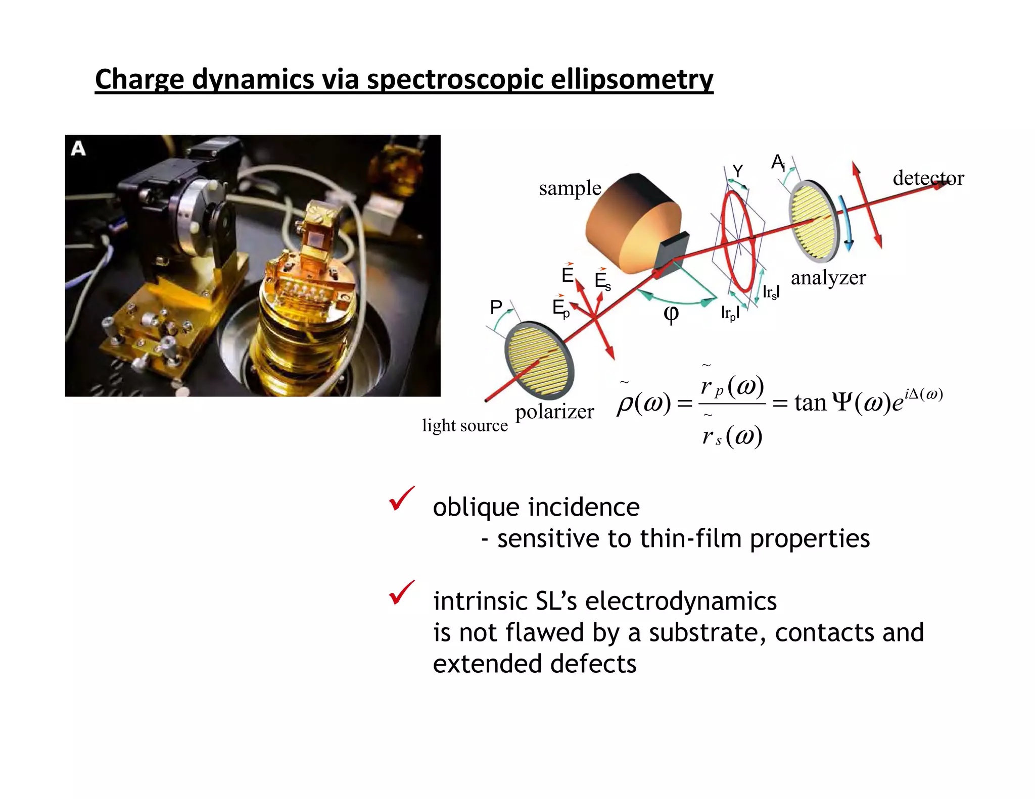
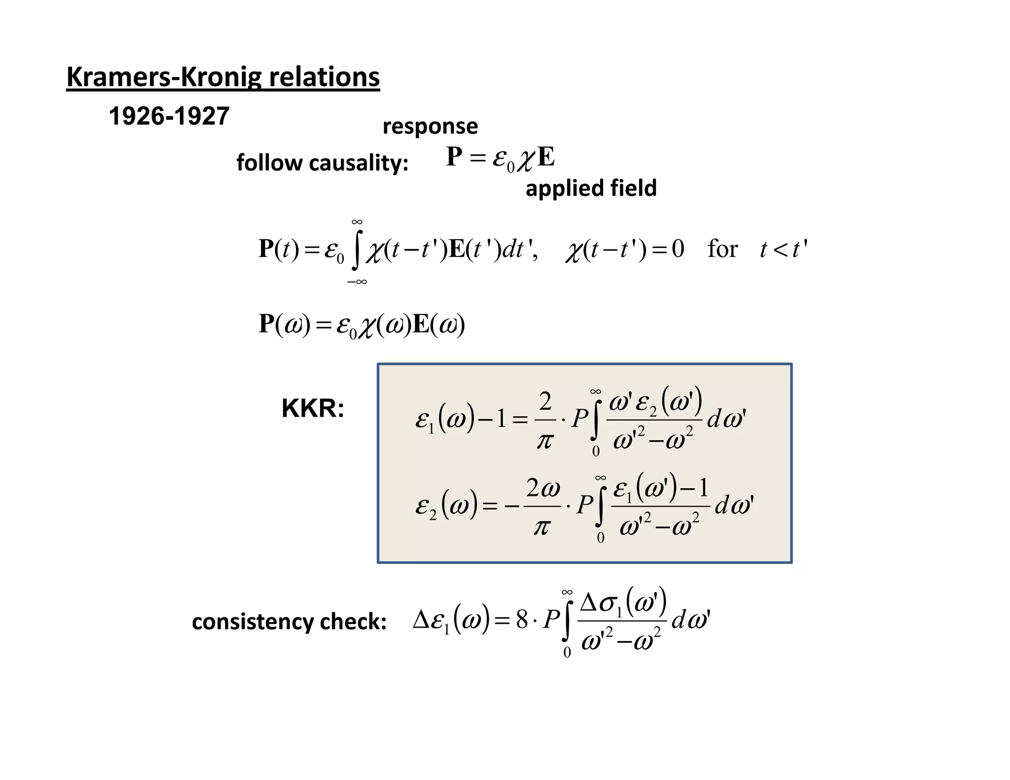
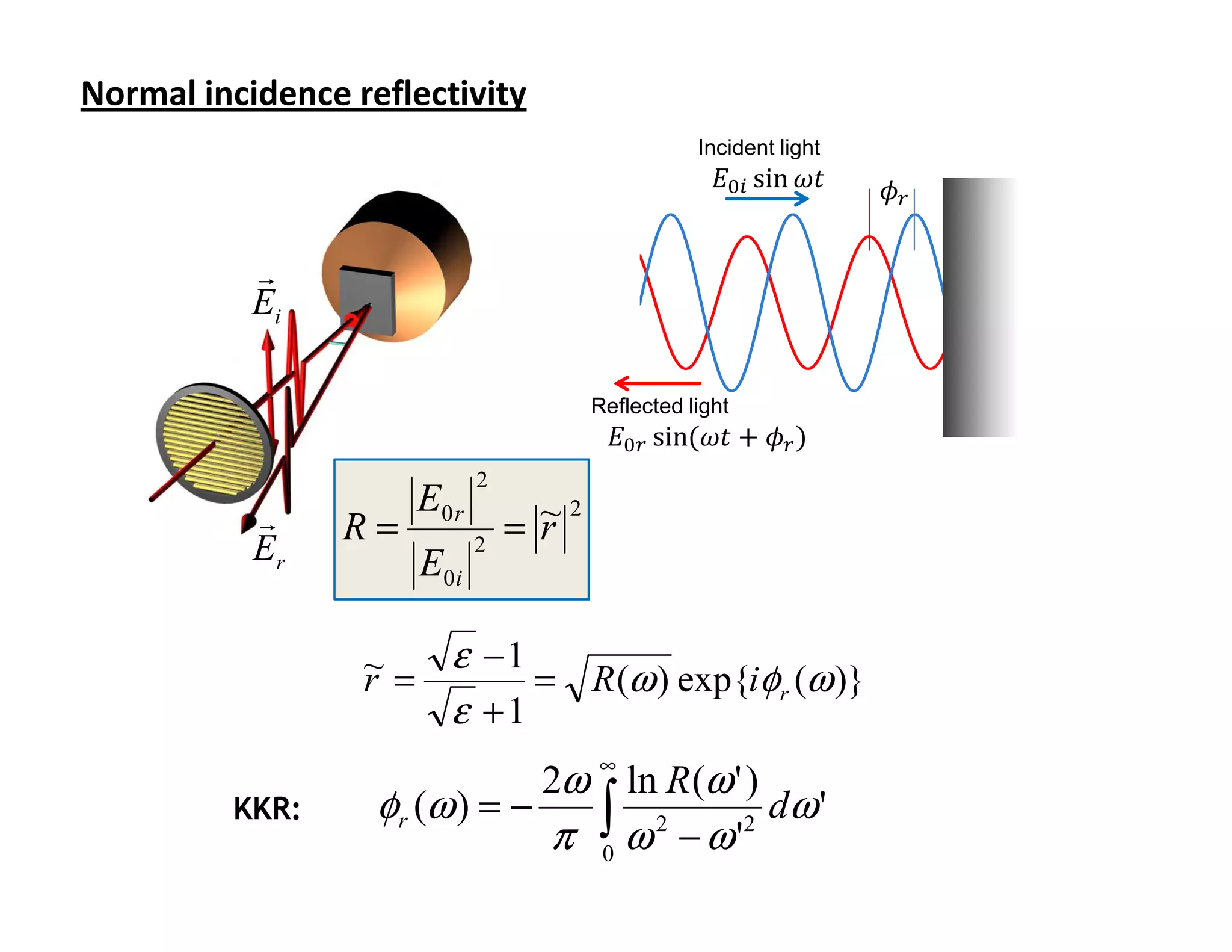
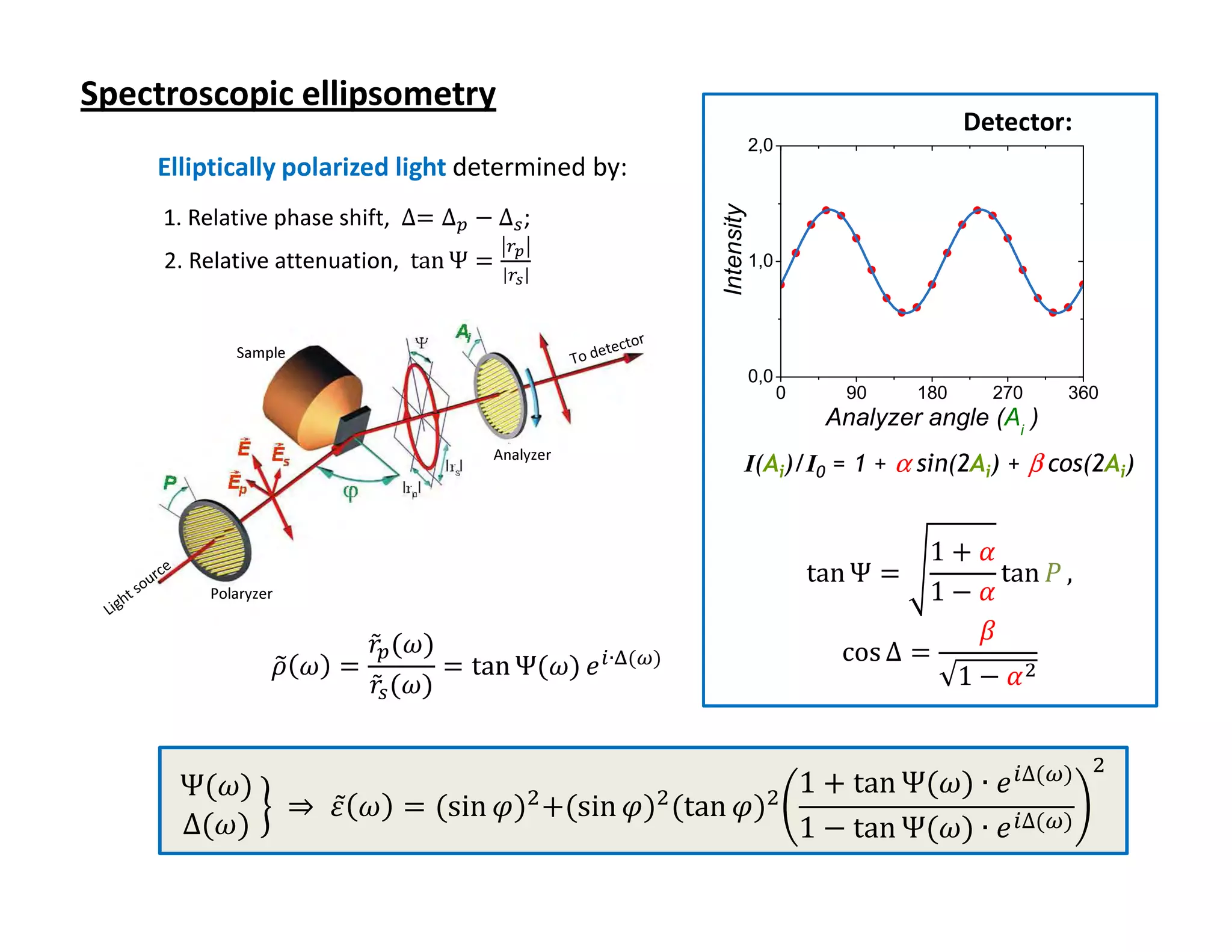
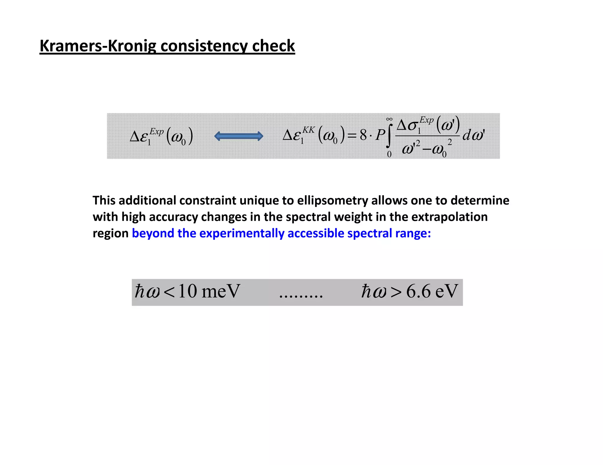
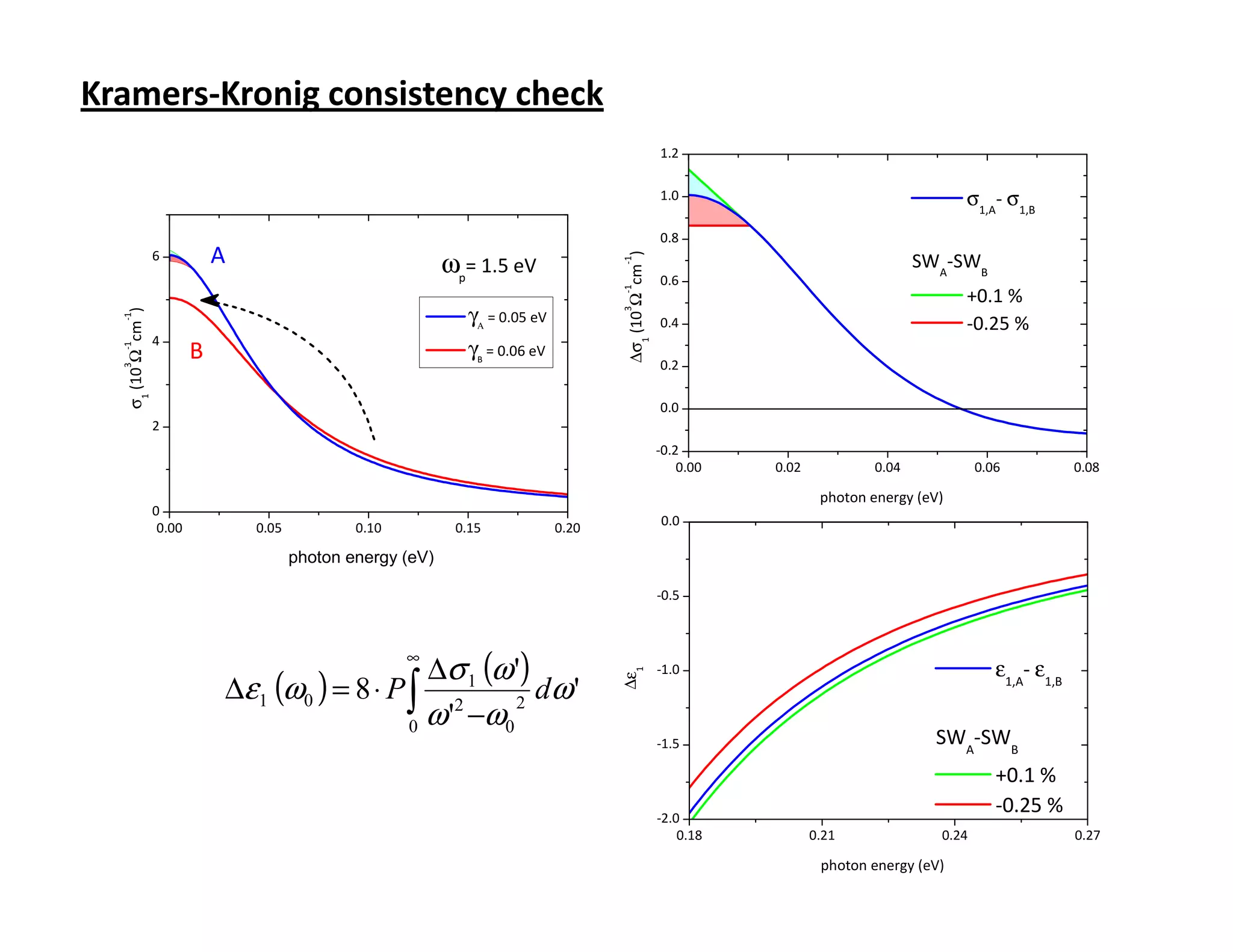
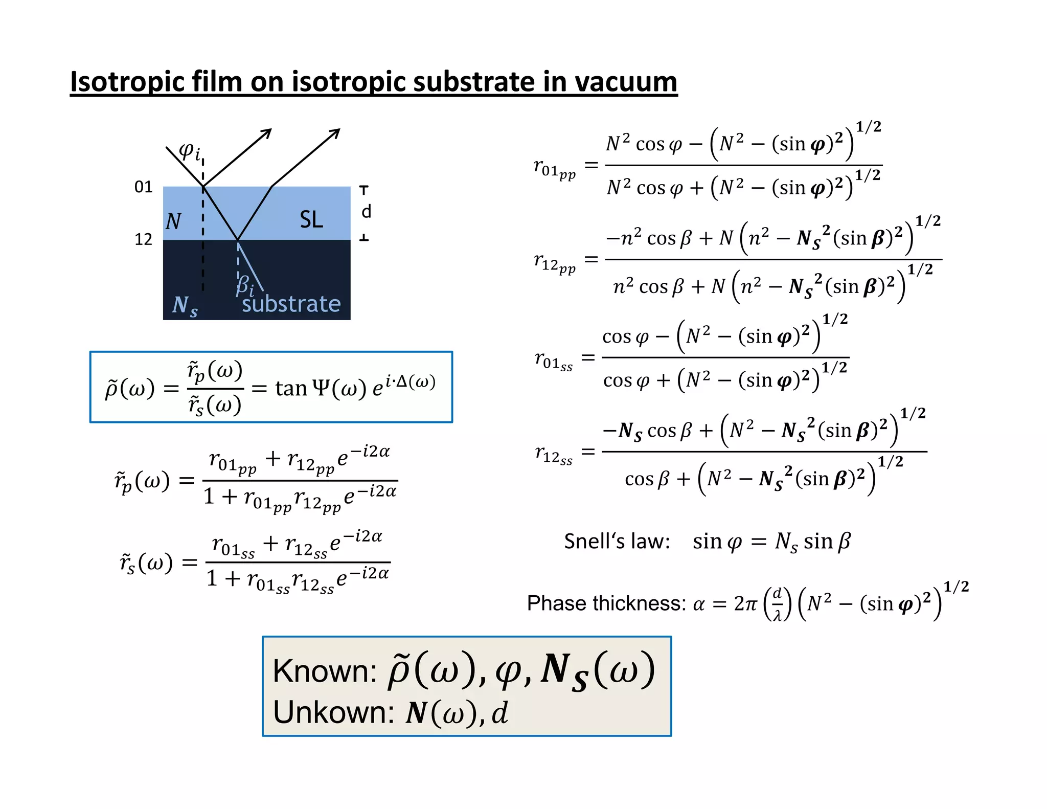
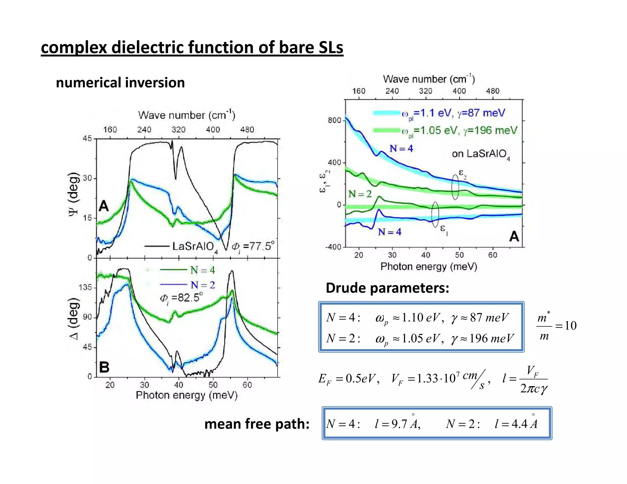
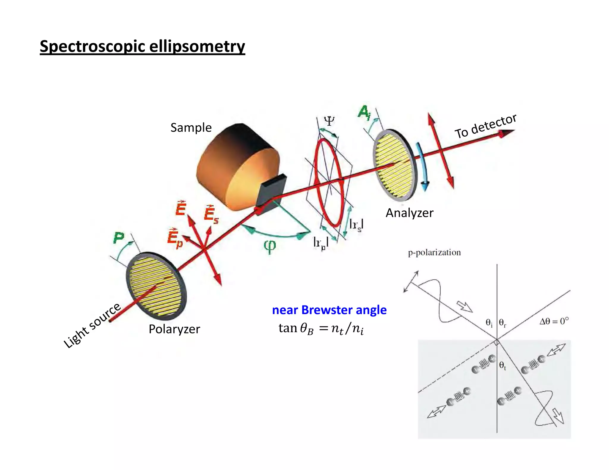
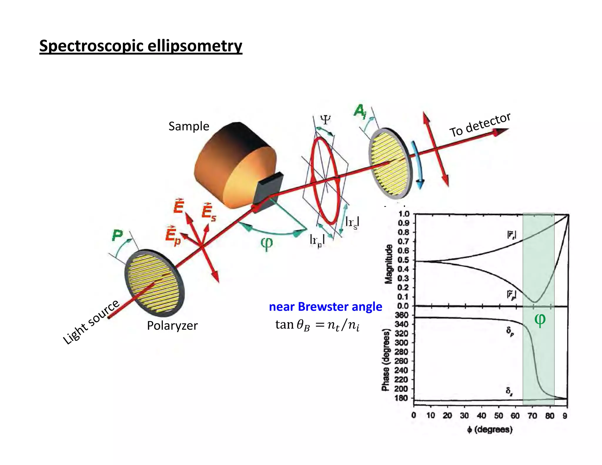
Spectroscopic ellipsometry is a technique for investigating the optical properties and electrodynamics of materials. It has several advantages over other optical techniques: 1) It provides an exact numerical inversion with no need for Kramers-Kronig transformations, allowing consistency checks. 2) Measurements are non-invasive and highly reproducible as they do not require reference samples. 3) It is very sensitive to thin film properties due to its ability to measure at oblique angles of incidence. 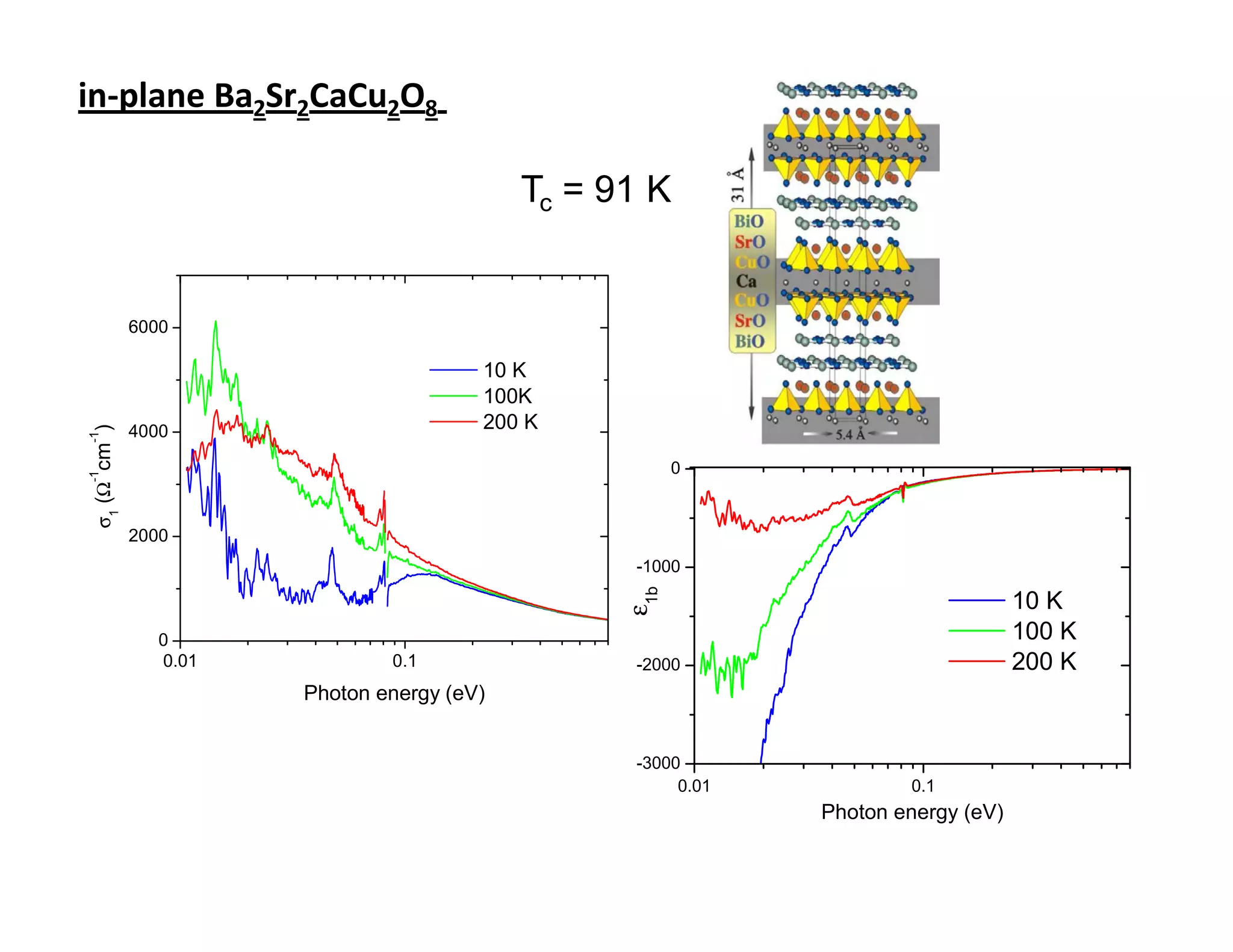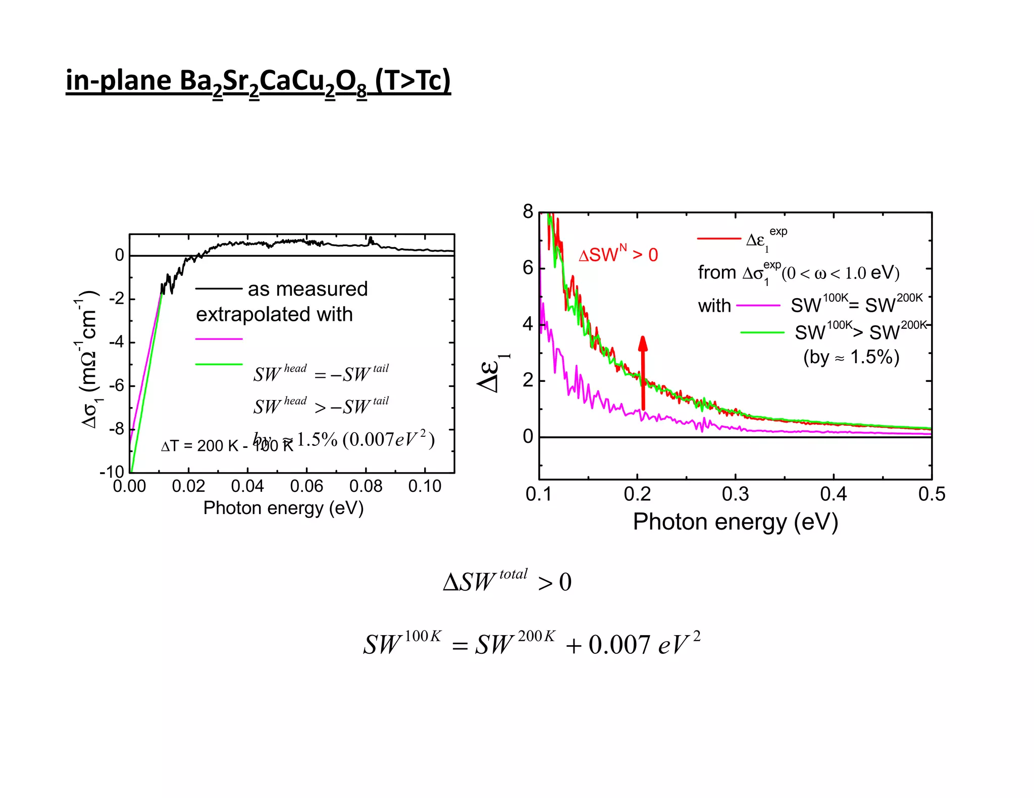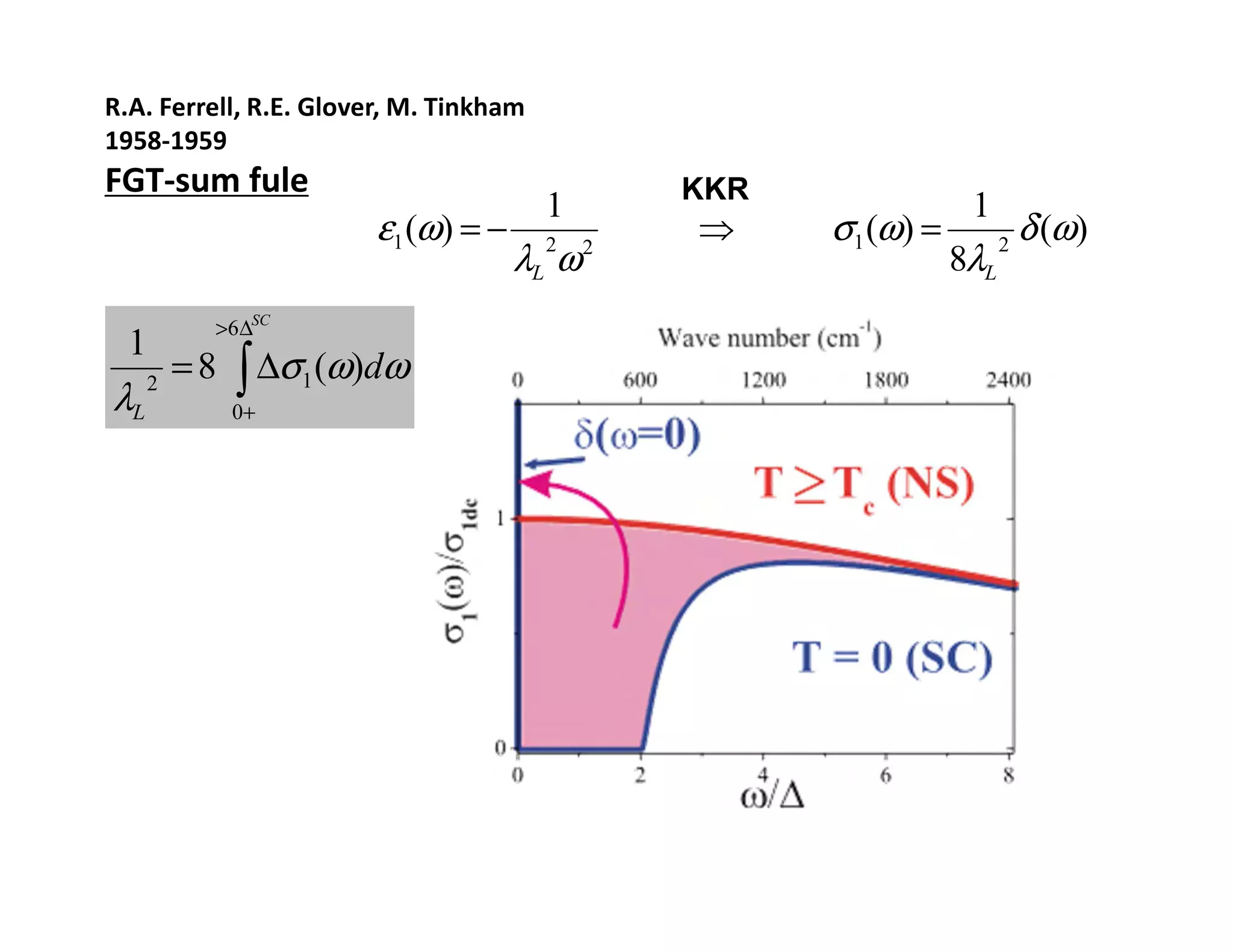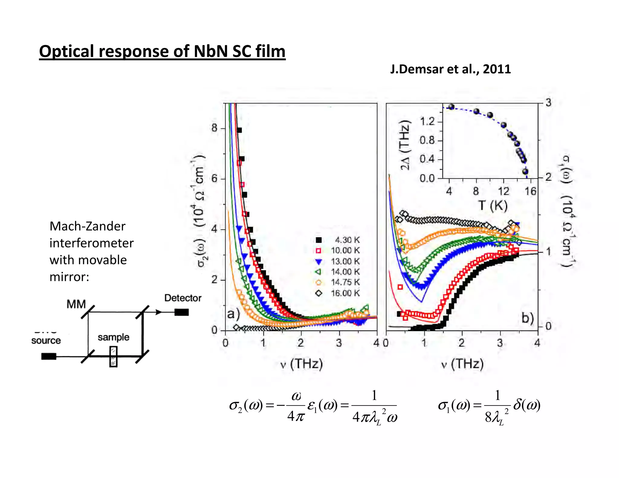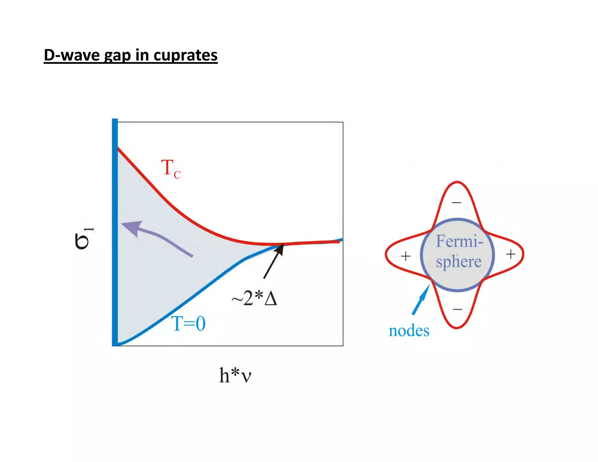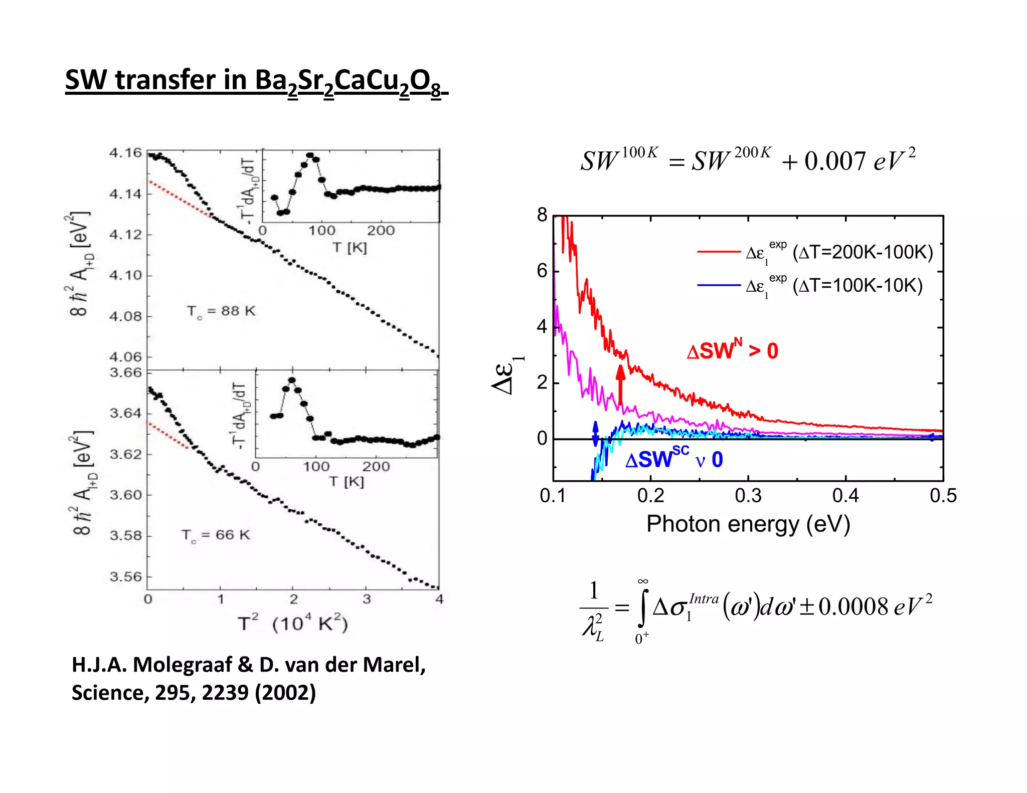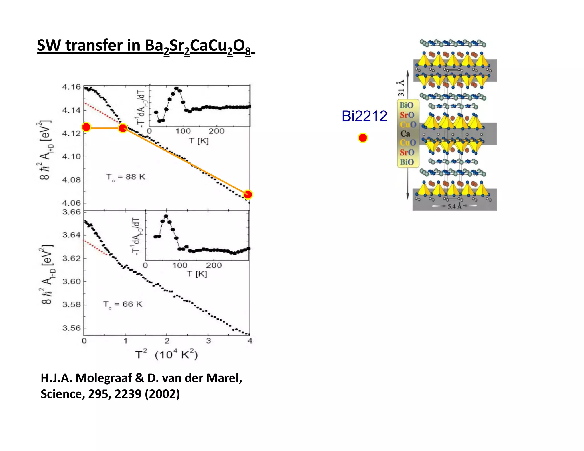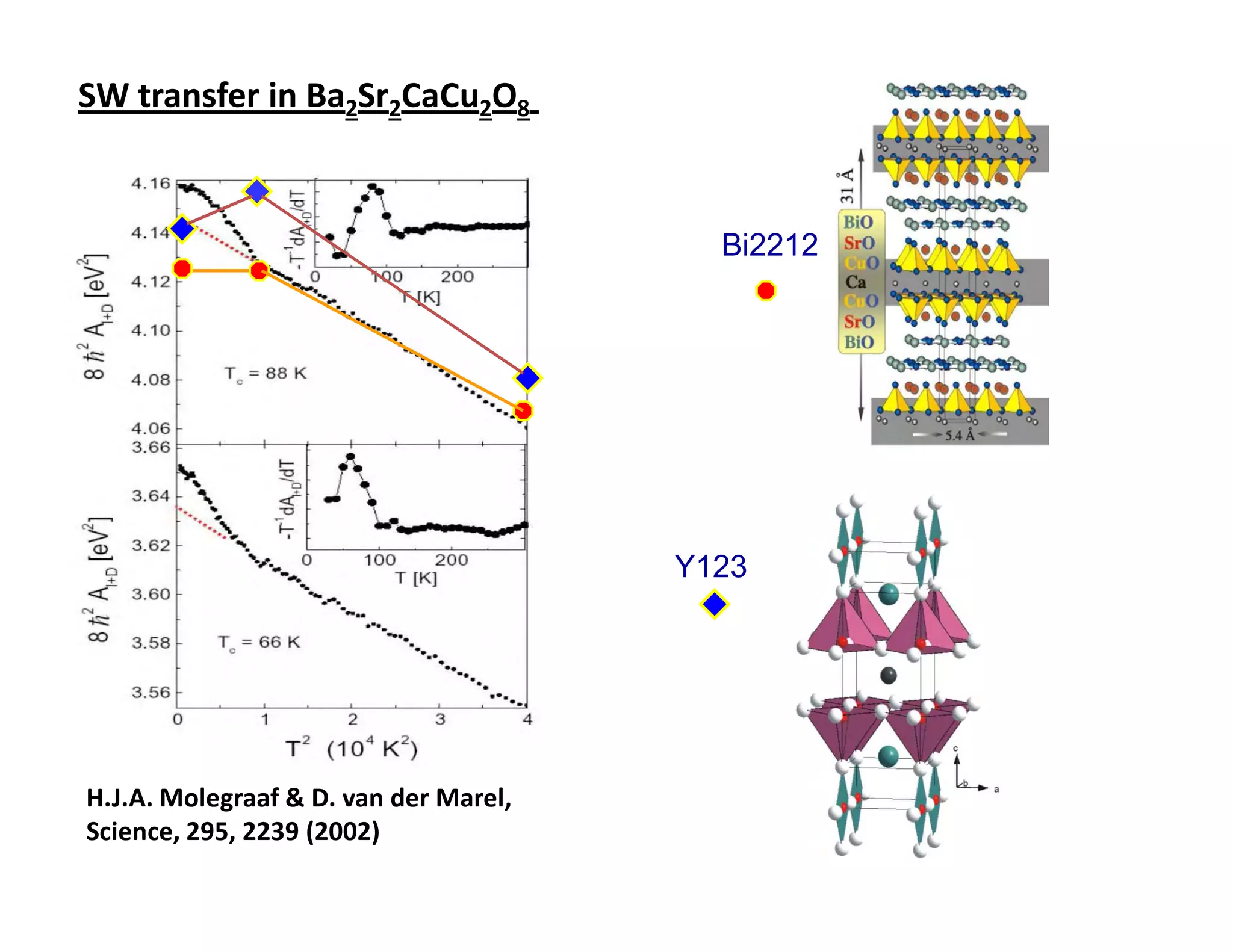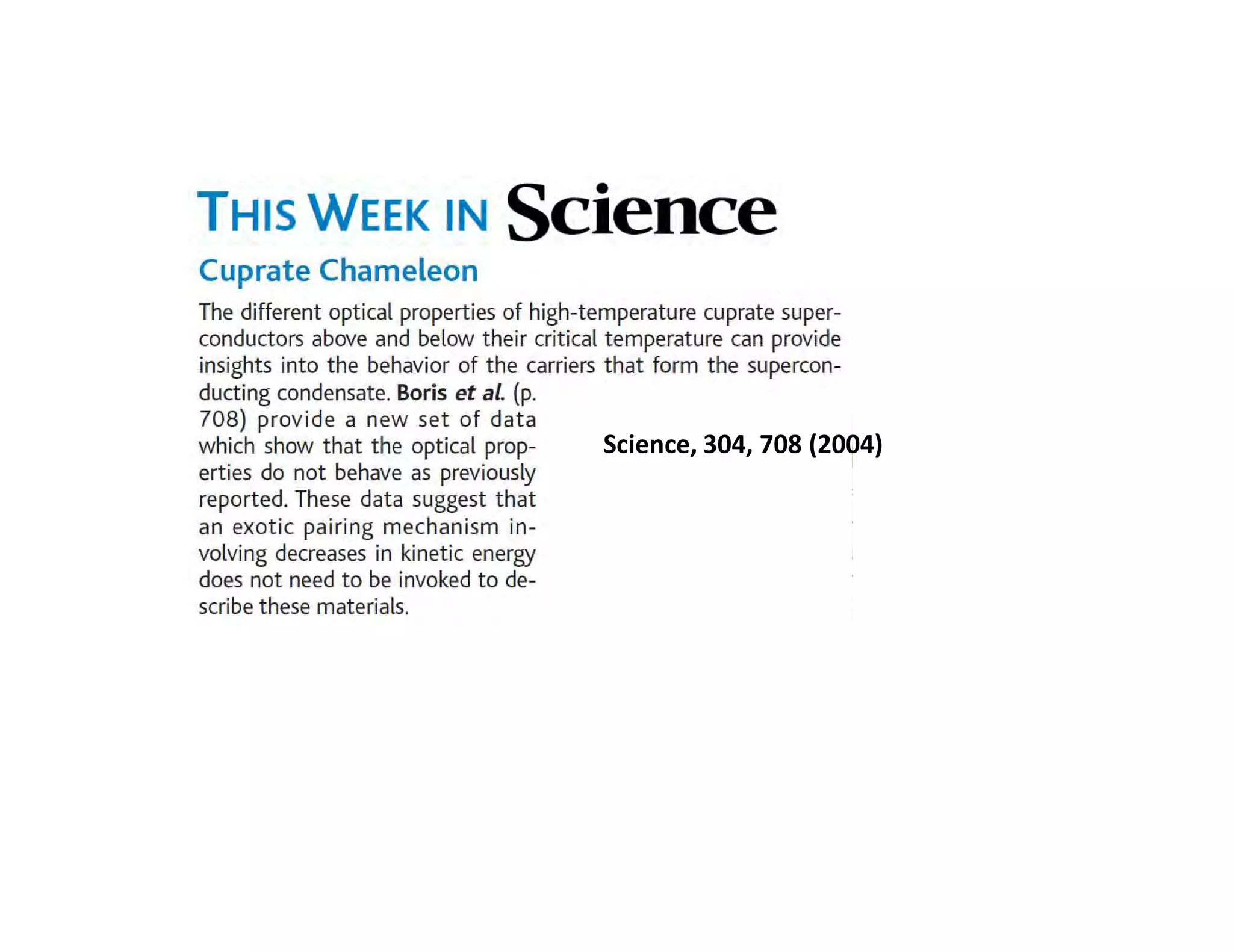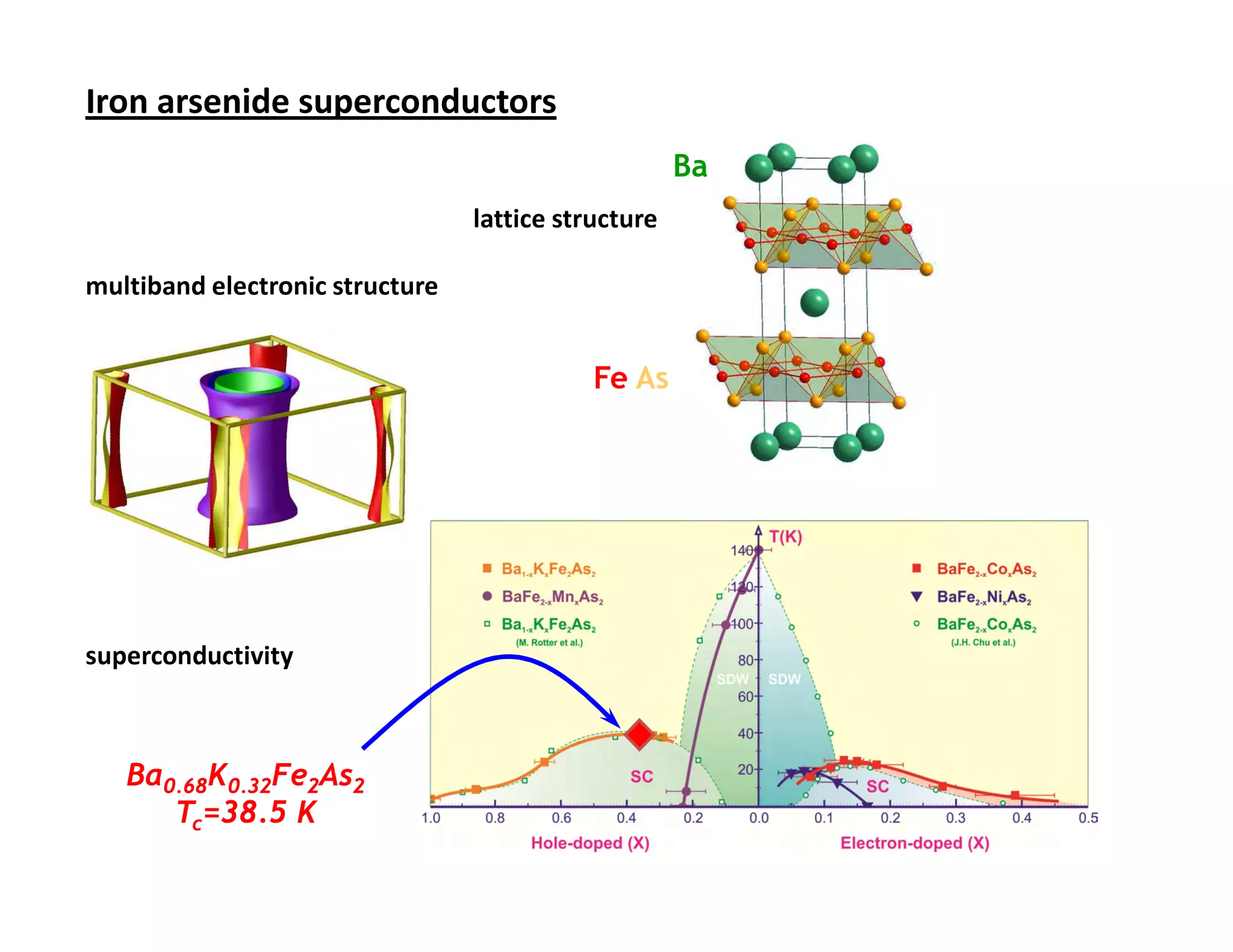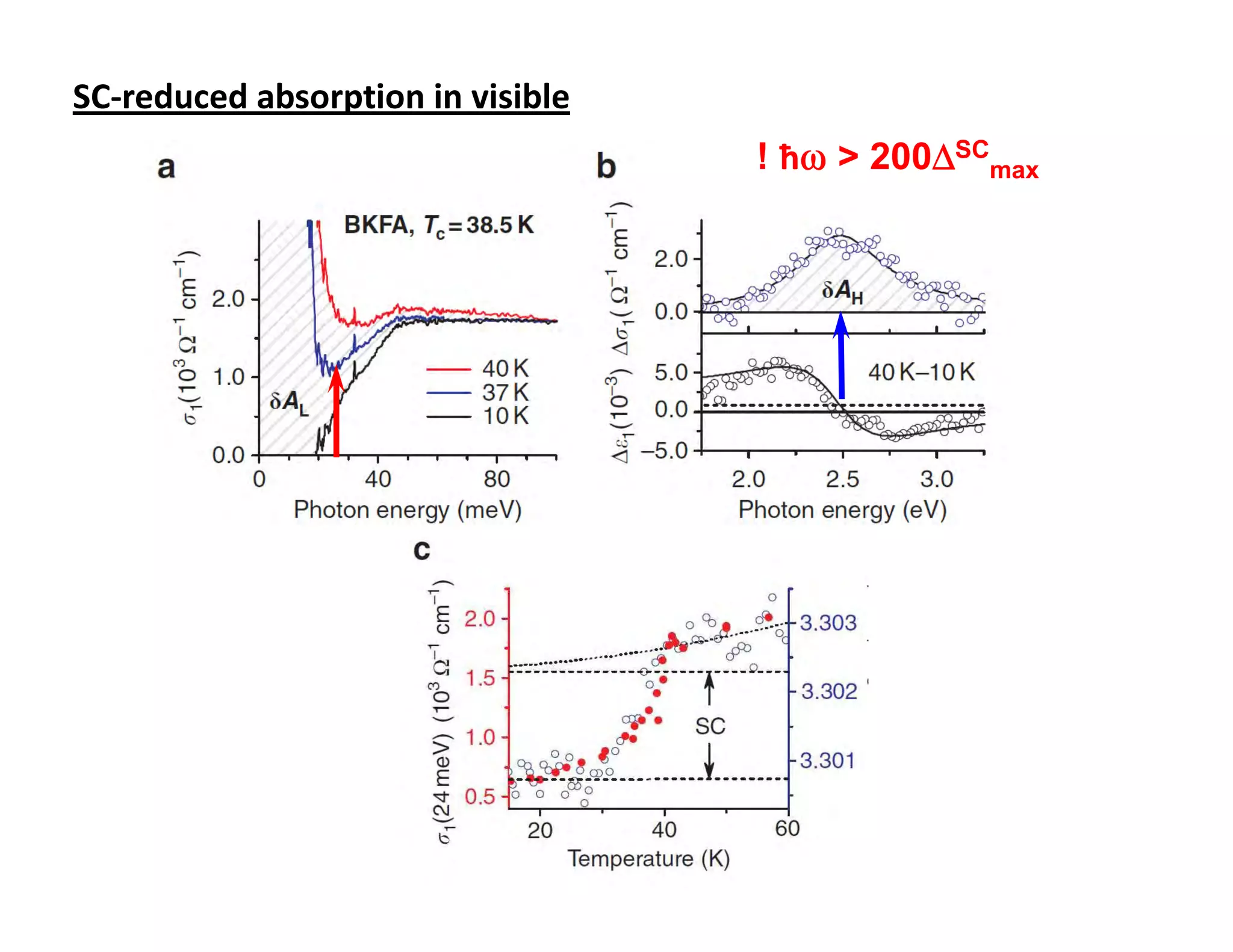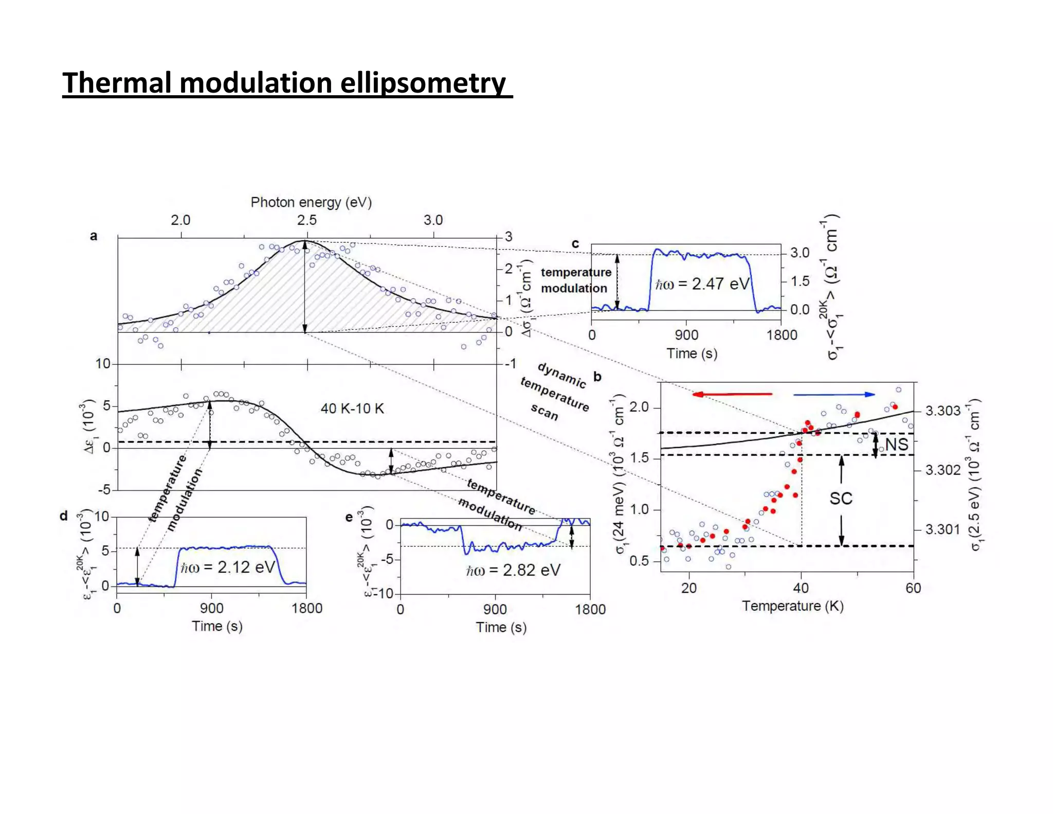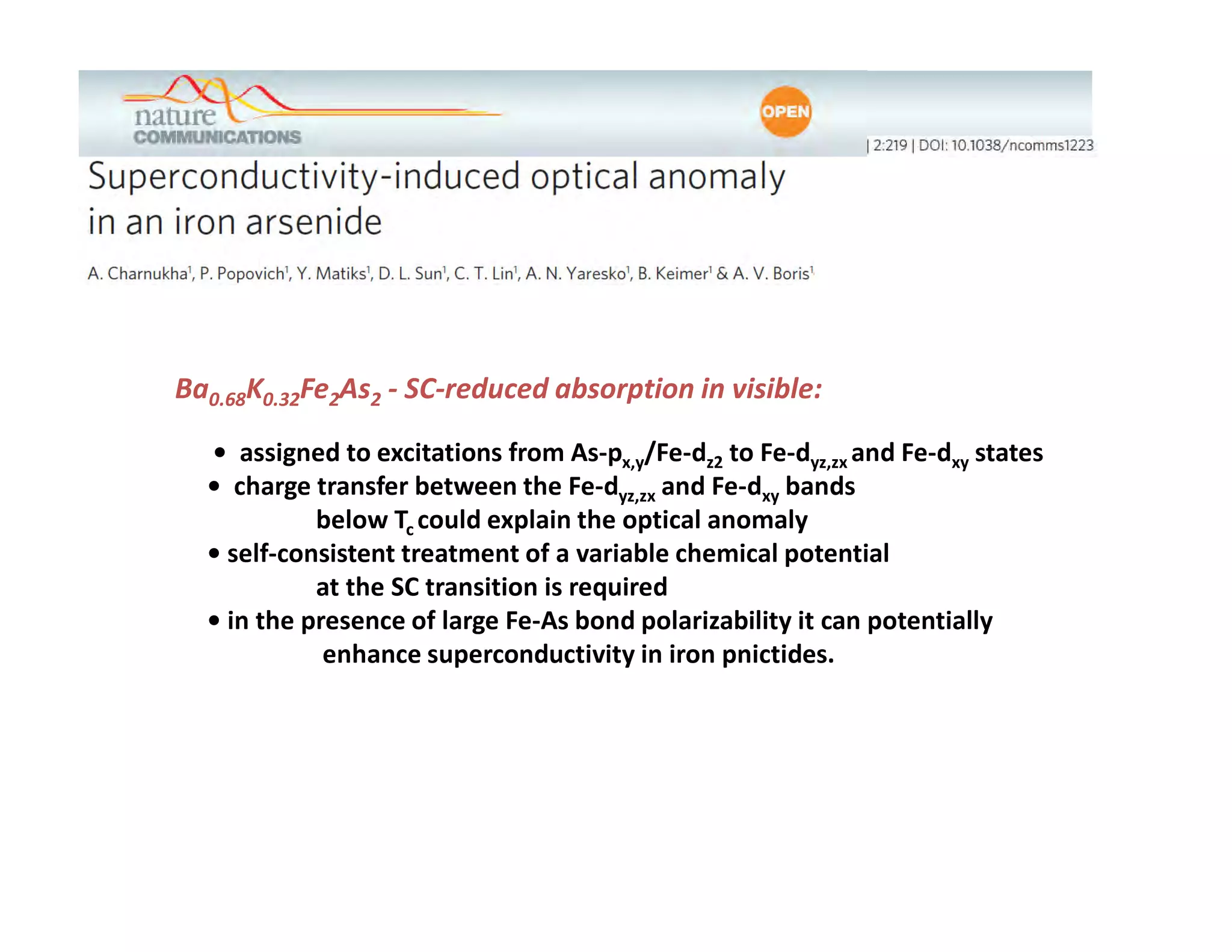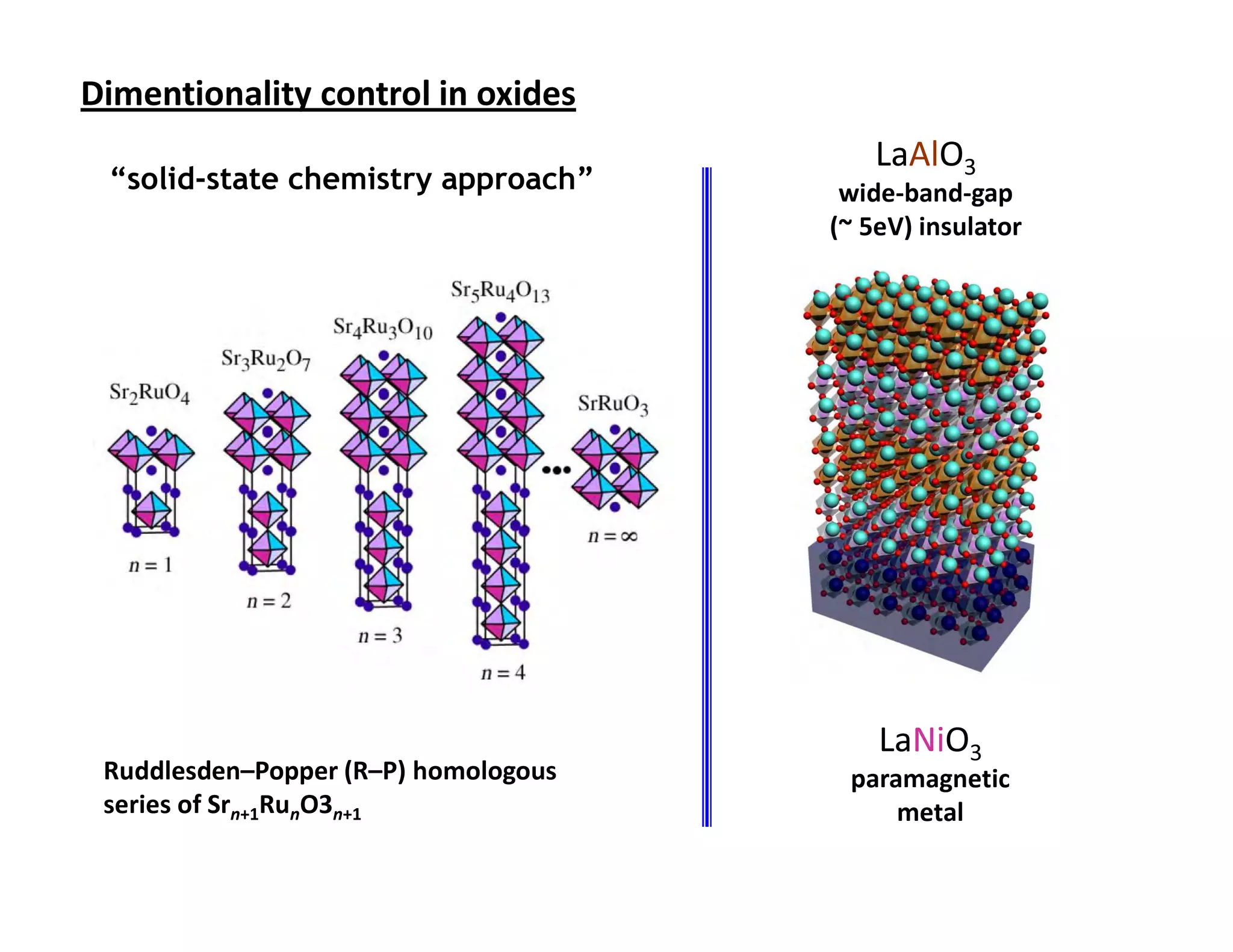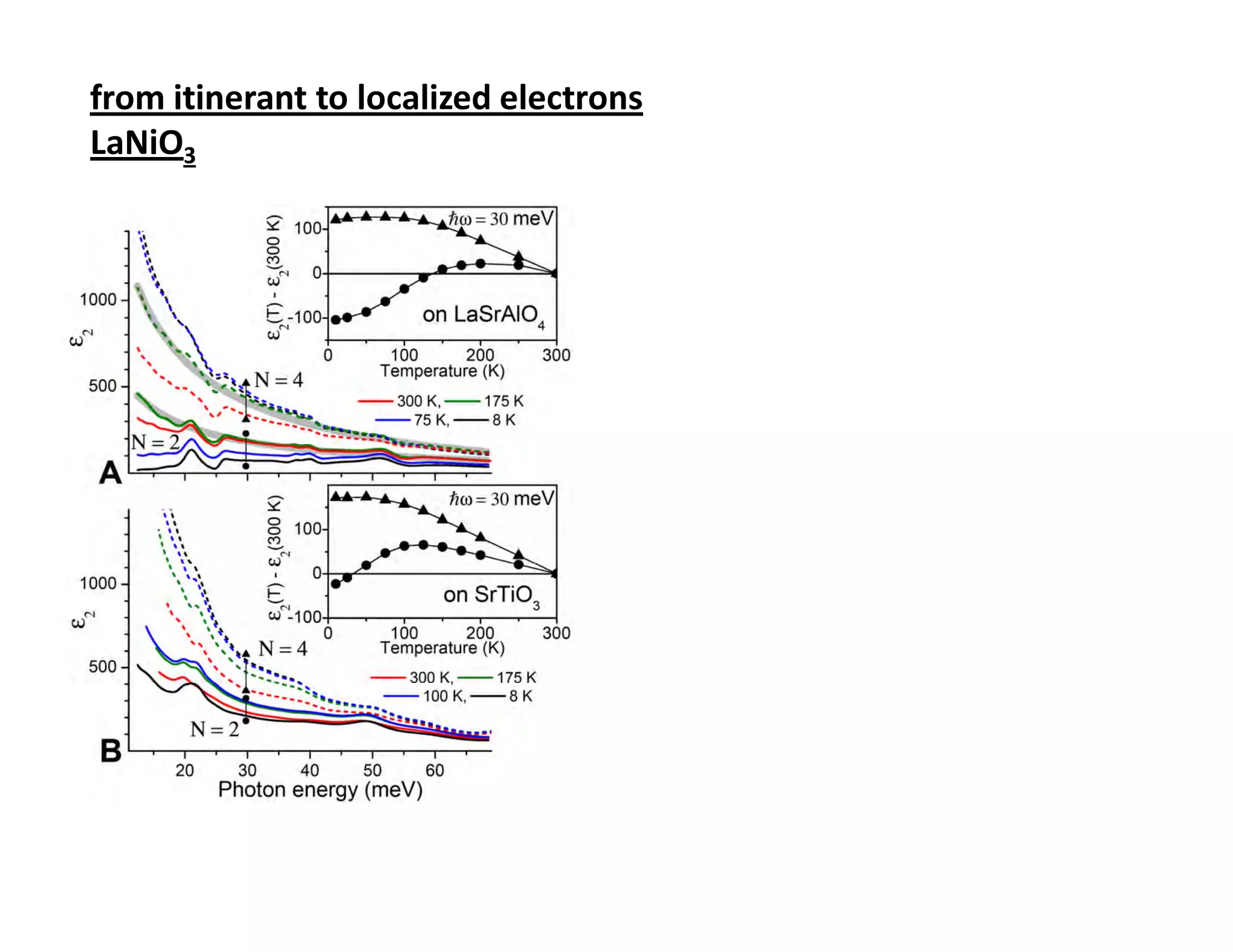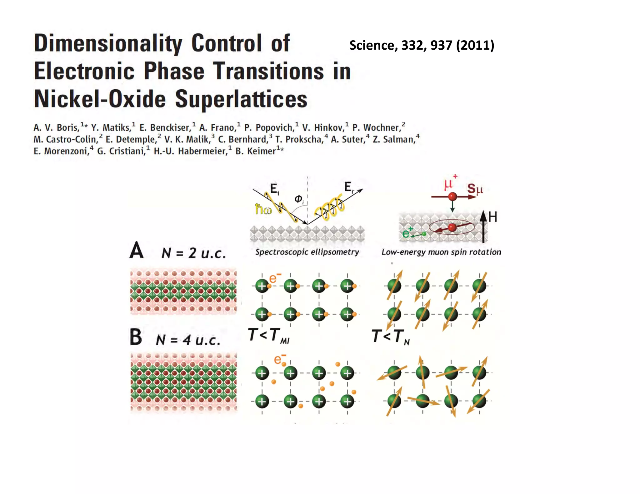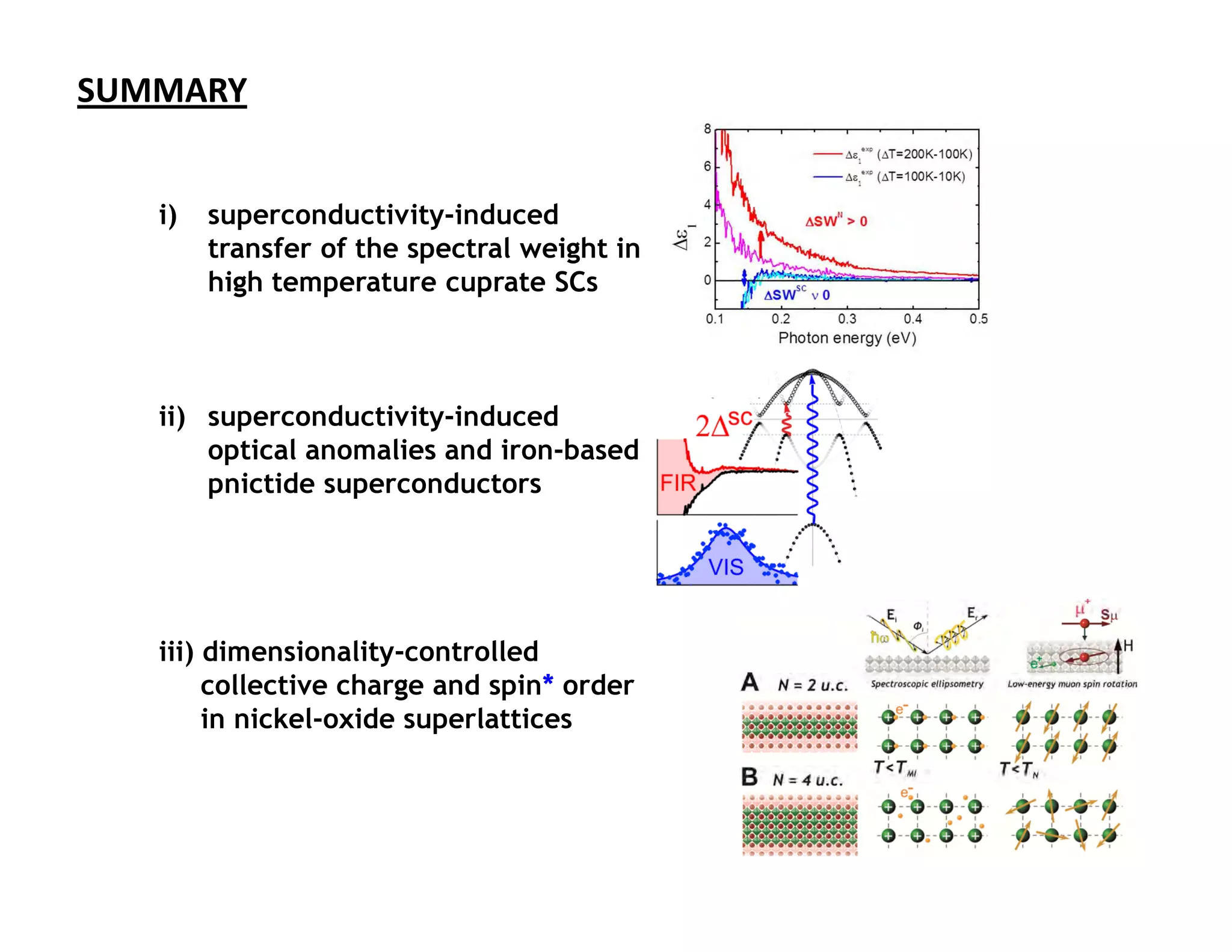Ellipsometry has been used to study phenomena like superconductivity in cuprates and pnictides by measuring changes in spectral weight, and collective charge ordering in oxide superlattices.

1. Alexander BORIS
Max Planck Institute for Solid State Research
Stuttgart
Spectroscopic ellipsometry:
application to electrodynamics
of correlated electron materials
and oxide superlattices.
September 1, 2011, Vancouver
MAX-PLANCK-UBC CENTRE FOR QUANTUM MATERIALS
International Summer School on Surfaces and Interfaces in Correlated Oxides

2. Outline Outline
• the complex dielectic function spectra -
one of the first steps in research of the
physical properties of a new material
• spectroscopic ellipsometry -
basic principles and experimental implementation
• advantages of ellipsometry - illustrative examples -
i) exact numerical inversion, no i) superconductivity-induced
Kramers-Kronig transformation, transfer of the spectral weight in
allows for K-K consistency check high temperature cuprate SCs
ii) no reference measurements, very ii) superconductivity-induced optical
accurate and highly reproducible anomalies and iron pnictide
superconductors
iii) oblique and variable angle of iii) dimensionality-controlled
incidence, very sensitive to collective charge and spin* order
thin-film properties in nickel-oxide superlattices
* combined with low-energy muons which serve as a sensitive
local probe of the internal magnetic field distribution

3. Outline Outline
• the complex dielectic function spectra -
one of the first steps in research of the
physical properties of a new material

4. Electromagnetic waves Electrodynamics of Solids
‫ܧ = ܧ‬଴ ݁ [௜(ఠ௧ିk‫ ݔ‬ାఋ)]

5. Dielectric polarization, susceptibility, pemittivity
Electrodynamics of Solids
ࡱ ࡼ
+ +q
- -
- -
Polarization
+
Electric field
- + ݈
- -
- + -q
-
ߤ ൌ ‫݈∙ݍ‬
Electric Ionic (phonon) Dipole moment
Polarization ࡼ ൌ ∑࢏ ࣆ࢏ ൌ ߝ଴ χ ࡱ
ࡼ
ࢿ ൌ 1 ൅ χ ൌ 1 ൅
ఌబ ࡱ

6. 4π
Electrodynamics of ∂E
∇× H = j + ε 0ε Solids
Maxwell’s equations for wave c ∂t
propagation in a conductor: ∂H
∇ × E = −µ0
∂t
 ∂E ∂ 2E 
⇒ ∇ × (∇ × E) = −∇ E = − µ0 σ
2
+ ε 0ε 2 
 ∂t ∂t 
plane wave : ‫ܧ = ܧ‬଴ ݁ [௜(ఠ௧ିk‫ ݔ‬ାఋ)] ⇒ k ଶ = ߤ଴ ݅߱ߪ + ߤ଴ ߝ଴ ߝ߱ଶ
4ߨ 1
SI → CGS: ߤ଴ → ଶ , ߝ଴ →
ܿ 4ߨ
ఠమ ସగ ఠ ସగ
k ଶ = ߝ+݅ ߪ , k ≡ N, Nଶ = ߝ + ݅ ߪ
௖మ ఠ ௖ ఠ
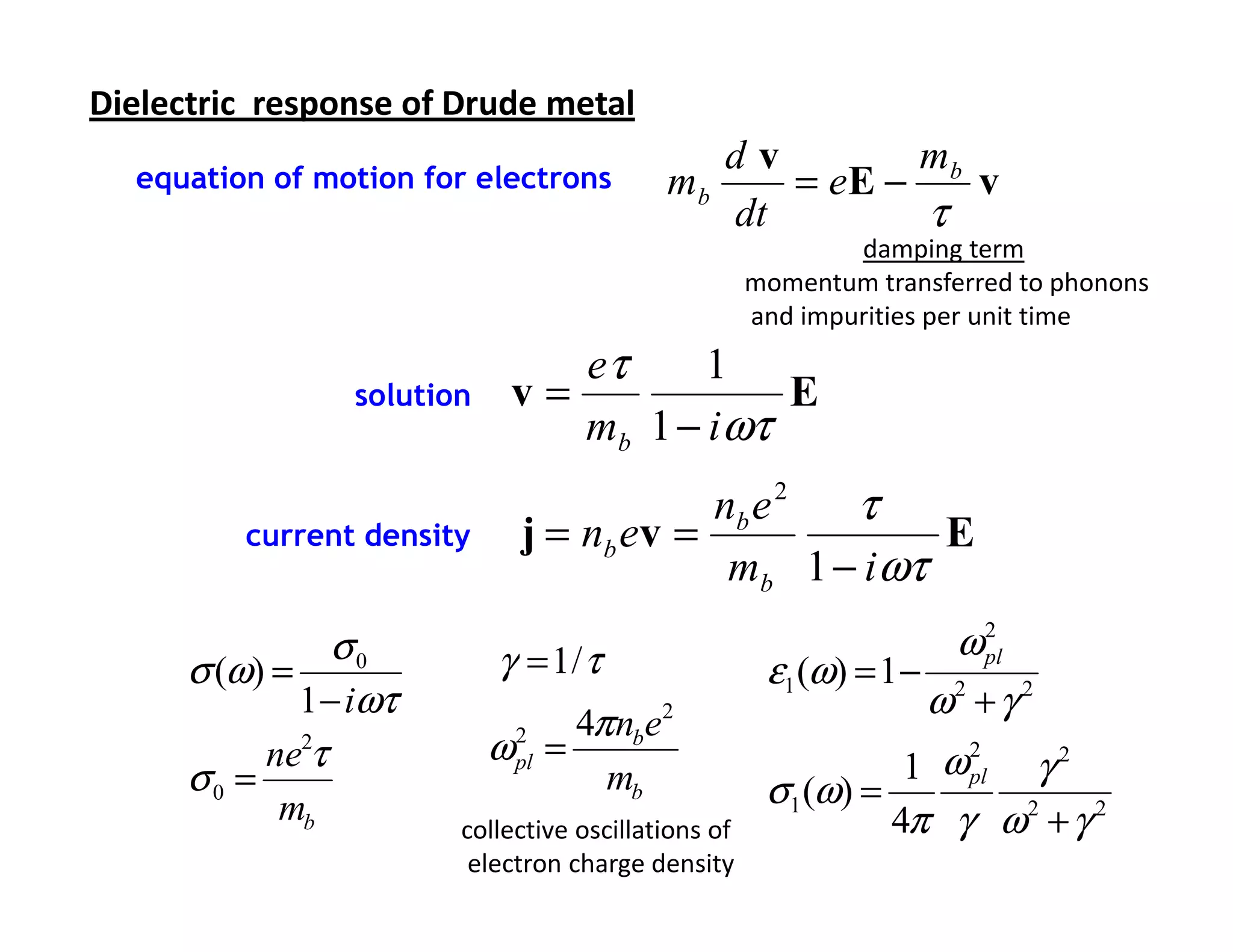
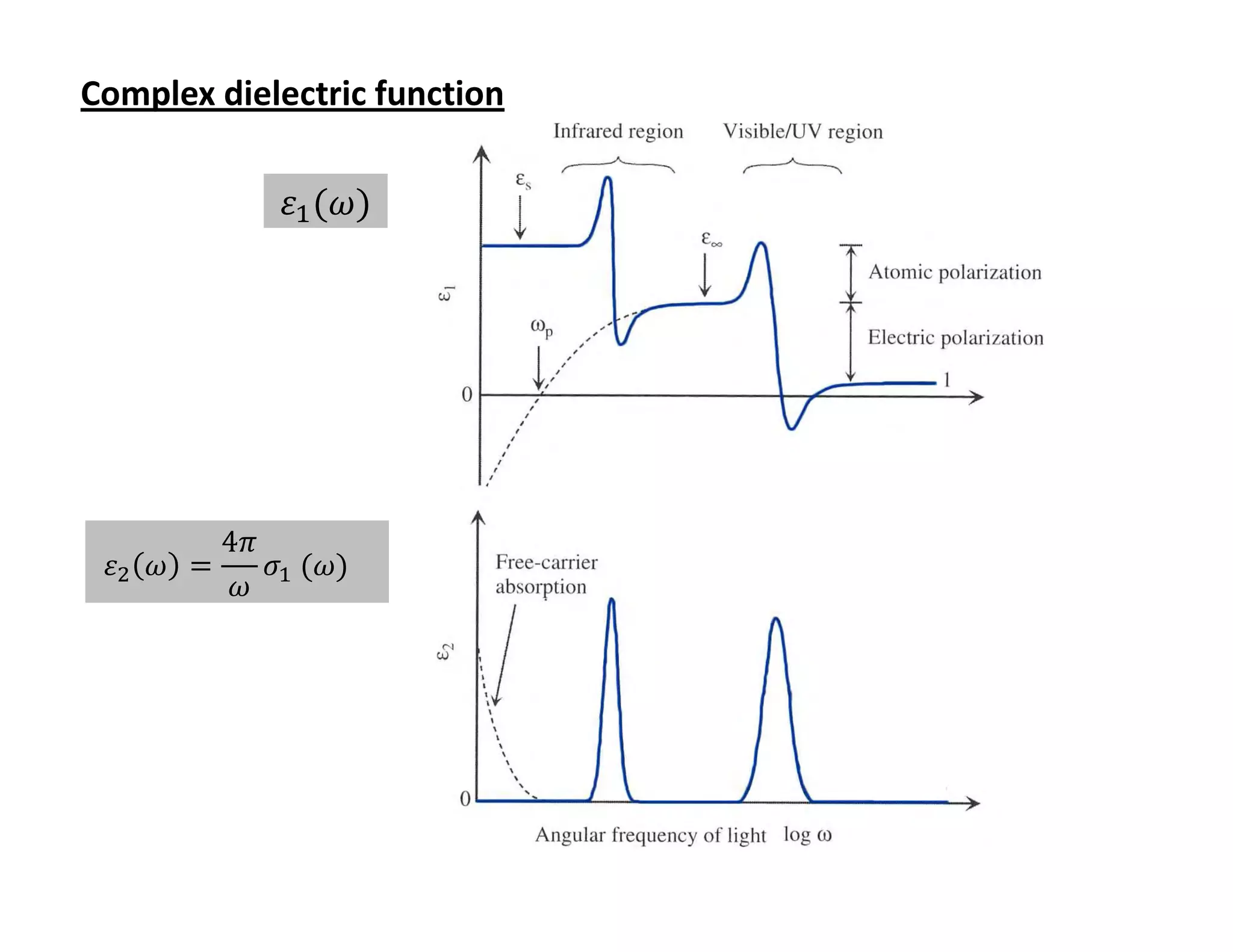
Complex dielectric function optical conductivity
ߝ̃ ߱ = ߝଵ (߱) + ݅ ∙ ߝଶ (߱) ߪ ߱ = ߪଵ ߱ + ݅ ∙ ߪଶ (߱)
෤
4ߨ
ߝଶ ߱ = ߪଵ (߱)
߱

7. Dielectric response of Drude metal
dv mb
equation of motion for electrons mb = eE − v
dt τ
damping term
momentum transferred to phonons
and impurities per unit time
eτ 1
solution v= E
mb 1 − iωτ
nb e 2 τ
current density j = nb e v = E
mb 1 − iωτ
σ0 γ = 1/ τ ω pl
2
σ (ω) = ε1 (ω) = 1 − 2 2
1 − iωτ ω +γ
4π nbe2
ne2τ ω pl =
2
ω pl γ 2
2
σ0 = mb σ1 (ω) =
1
mb collective oscillations of 4π γ ω 2 + γ 2
electron charge density

8. Complex dielectric functionElectrodynamics of Solids
ߝଵ (߱)
4ߨ
ߝଶ ߱ = ߪ (߱)
߱ ଵ

9. Optical sum rules: ∞
Spectral Weight and Sum Rules π ne e 2
f-sum rule: SW (0, ∞) = ∫ σ 1 (ω )dω = = const
0
2me
݊௘ - total number of electrons in the system, ݉௘ - free electron mass
D.Y. Smith and E. Shiles,
PRB 17, (1978) 4689-4694
Ω
= 2 Al ∫ σ (ω )dω
2m
neff
πe N 0
Ω
ω pl
2
π nb e 2
intra-band spectral weight: SW intra
(0, ∞) = = = f (T ) ≠ const
8 2mb

10. Kramers-Kronig relations
1926-1927 response
follow causality: P = ε 0 χ E
applied field
∞
P(t ) = ε 0 ∫ χ (t − t ' )E(t ' )dt ', χ (t − t ' ) = 0 for t < t '
−∞
P(ω) = ε 0 χ (ω)E(ω)
∞
ω ' ε 2 (ω ')
ε 1 (ω ) − 1 =
2
KKR: ⋅ P∫ dω '
π 0
ω ' −ω
2 2
2ω
∞
ε 1 (ω ') − 1
ε 2 (ω ) = − ⋅ P∫ dω '
π 0
ω ' −ω
2 2
∆σ 1 (ω ')
∞
consistency check: ∆ε 1 (ω ) = 8 ⋅ P ∫ 2 dω '
0
ω ' −ω 2

11. Normal incidenceReflectivity by normal incidence
reflectivity
Incident light
‫ܧ‬଴௜ sin ߱‫ݐ‬ ߶௥
r
Ei
Reflected light
‫ܧ‬଴௥ sinሺ߱‫ ݐ‬൅ ߶௥ ሻ
2
E0 r ~2
r R= =r
Er E0 i
2
~ = ε − 1 = R (ω ) exp{iφ (ω )}
r
ε +1
r
∞
2ω ln R (ω ' )
KKR: φr (ω ) = − ∫ ω 2 − ω ' 2 dω '
π 0

12. Outline Outline
• spectroscopic ellipsometry -
basic principles and experimental implementation

13. Analogy with electric circuit electric circuit admittance
Analogy with impedance
Lissajous figure
a b resistance & reactance
(complex impedance)
X Y
Z = R+iωL
R Vmaxsinωt
ϕ Imaxsin(ωt-ϕ)
L Vmax
Imax
ϕ= arctan(ωL/R)=
= arcSin(a/b)
Time

14. Polarization of light Electrodynamics of Solids
ࡱ-field vector ࡱ = ࡱ࢞ + ࡱ࢟
Y
Linear polarization
phase delay ߮=0 X
Y
Curcular polarization
phase delay ߮=ߨ/2
X
Y
Elliptical polarization Ψ
‫ܧ‬௫
phase delay ߮=0.35·2ߨ
X
‫ܧ‬௬

15. Spectroscopic ellipsometry
Sample
Analyzer
near Brewster angle
Polaryzer tan ߠ஻ = ݊௧ ⁄݊௜

16. Spectroscopic ellipsometry
Sample
Analyzer
near Brewster angle
Polaryzer tan ߠ஻ = ݊௧ ⁄݊௜ ϕ

17. Spectroscopic ellipsometry
Detector:
2,0
Elliptically polarized light determined by:
Intensity
1. Relative phase shift, ∆= ∆௣ − ∆௦ ;
௥೛
2. Relative attenuation, tan Ψ = 1,0
௥ೞ
Sample
0,0
0 90 180 270 360
Analyzer angle (Ai )
Analyzer
I(Ai)/I0 = 1 + α sin(2Ai) + β cos(2Ai)
1+ߙ
tan Ψ = tan ܲ ,
Polaryzer 1−ߙ
̃
‫ݎ‬௣ (߱) ߚ
෤
ߩ ߱ = = tan Ψ(߱) ݁ ௜∙୼(ఠ) cos Δ =
̃
‫ݎ‬௦ (߱) 1 − ߙଶ
1 + tan Ψ(߱) ∙ ݁ ௜∆(ఠ)
ଶ
Ψ(߱)
ൠ ⇒ ߝ̃ ߱ = (sin ߮)ଶ +(sin ߮)ଶ (tan ߮)ଶ
Δ(߱) 1 − tan Ψ(߱) ∙ ݁ ௜∆(ఠ)

18. Spectroscopic ellipsometry
Paul Drude
ellipsometer
~ 1890
2007

19. ANKA Synchrotron, Karlsruhebeamline at ANKA
IR IT
IR-1 beamline
Y.-L. Mathis, B. Gasharova, D. Moss
Current: 80 -180 mA
lifetime: 12-23 hours

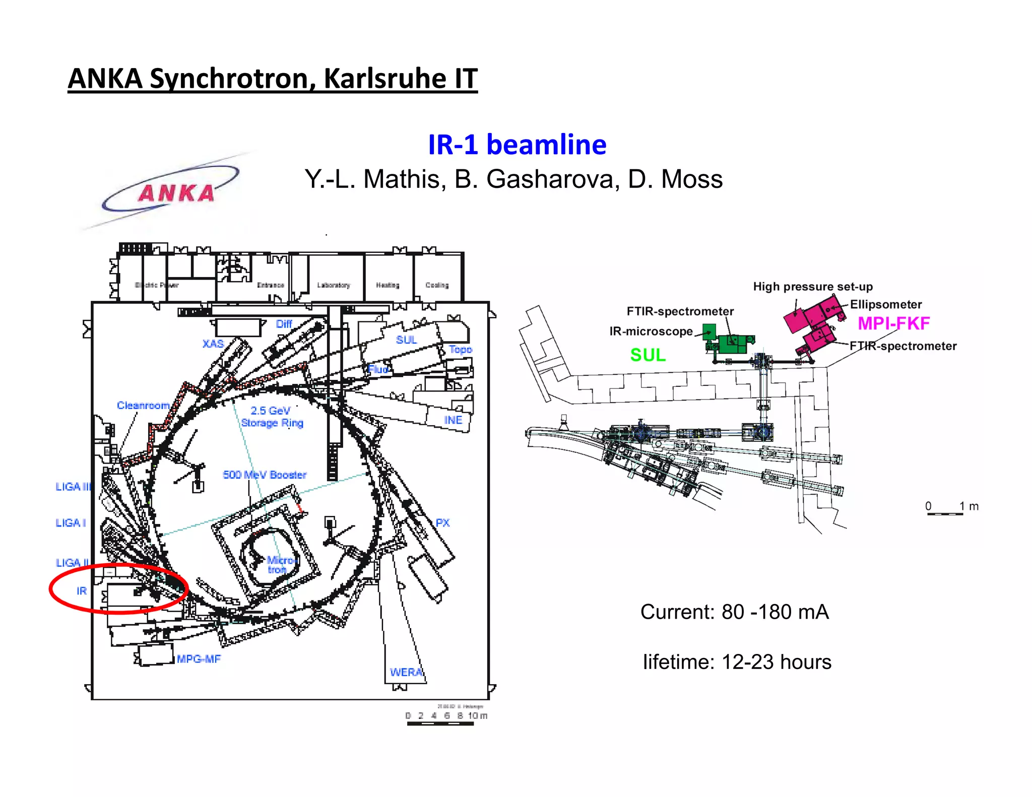
20. ANKA Synchrotron, Karlsruhebeamline at ANKA
IR IT
IR-1 beamline
Y.-L. Mathis, B. Gasharova, D. Moss
1.5
Magnetic Field [T]
Magnetic profile
1.0
of a dipole
0.5 Edge and dipole
Spatial distribution radiation in the visible
from the edge at
0.0
3 m from the source
(calculated for 100µm) 1.0m 0.5 0.0 -0.5 -1.0
Position on particle trajectory [m]
Photons/s/.1%bw/mm^2 x10
40 150
20
at λ=10 µm
y [mm]
100
0
-20 50
-40mm
9
0
-40mm -20 0 20 40
x [mm]

21. wide-band spectroscopic ellipsometry THz to UV
Ellipsometry: from
ANKA Synchrotron
edge radiation
1m 10m 100m 1 eV 6.2
0.2 THz 1 2
far-IR mid-IR near-IR UV
10 100 1000 10000 cm-1
near-IR to deep-UV
far-IR homebuilt ellipsometer spectroscopic
at ANKA IR1- beam line, ellipsometer (VASE)
@ Karlsruhe IT Woollam Co., @ MPI-FKF
IR homebuilt ellipsometer
based on Bruker 66v/S FTIR
spectrometer, @ MPI-FKF

22. wide-band spectroscopic ellipsometry THz to UV
Ellipsometry: from
ANKA Synchrotron
edge radiation
1m 10m 100m 1 eV 6.2
0.2 THz 1 2
far-IR mid-IR near-IR UV
10 100 1000 10000 cm-1
near-IR to deep-UV
far-IR homebuilt ellipsometer spectroscopic
at ANKA IR1- beam line, ellipsometer (VASE)
@ Karlsruhe IT Woollam Co., @ MPI-FKF
IR homebuilt ellipsometer
based on Bruker 66v/S FTIR
spectrometer, @ MPI-FKF

23. Outline Outline
• advantages of ellipsometry -
i) exact numerical inversion, no
Kramers-Kronig transformation,
allows for K-K consistency check
ii) no reference measurements, very
accurate and highly reproducible
iii) oblique and variable angle of
incidence, very sensitive to
thin-film properties

24. Outline Outline
• advantages of ellipsometry - illustrative examples -
i) exact numerical inversion, no i) superconductivity-induced
Kramers-Kronig transformation, transfer of the spectral weight in
allows for K-K consistency check high temperature cuprate SCs

25. Kramers-Kronig consistency check
∆σ 1Exp (ω ')
∞
∆ε 1Exp (ω0 ) ∆ε KK
(ω0 ) = 8 ⋅ P ∫ 2 2 dω '
0 ω ' −ω0
1
This additional constraint unique to ellipsometry allows one to determine
with high accuracy changes in the spectral weight in the extrapolation
region beyond the experimentally accessible spectral range:
hω < 10 meV ......... hω > 6.6 eV

26. T-dependent Drude ω pl π e 2 nb
2
SW Drude = =
8 2 mb
σDC
γ (T1 ) > γ (T2 ) γ2
σ1 (ω) = σ DC
T1 > T2
ω2 + γ 2
0
ω pl
2
ε1 (ω) = ε ∞ − 2 2
-20
ε1
ω +γ
-40
0.0 0.5 1.0 1.5 2.0
hν (eV)

27. T-dependent Drude SW ω pl π e 2 nb
2
SW Drude = =
8 2 mb
electron correlation effects
σDC
UHB
Daniel Khomslii’s lecture
0
nb
= f (T ) ≠ const
-20 mb
ε1
-40
0.0 0.5 1.0 1.5 2.0
hν (eV)

28. Kramers-Kronig consistency check
1.2
1.0 σ1,A- σ1,B
0.8
A ωp= 1.5 eV
∆σ1 (10 Ω cm )
6 SWA-SWB
-1
0.6
-1
+0.1 %
γΑ = 0.05 eV
3
σ1 (10 Ω cm )
-1
0.4 -0.25 %
4
γB = 0.06 eV
-1
B 0.2
3
0.0
2
-0.2
0.00 0.02 0.04 0.06 0.08
photon energy (eV)
0
0.00 0.05 0.10 0.15 0.20 0.0
photon energy (eV)
-0.5
∆σ (ω ')
∞
ε1,A- ε1,B
∆ε 1 (ω0 ) = 8 ⋅ P ∫ 2 1 2 dω '
-1.0
∆ε1
0 ω ' −ω0
-1.5 SWA-SWB
+0.1 %
-2.0
-0.25 %
0.18 0.21 0.24 0.27
photon energy (eV)

29. in-plane Ba2Sr2CaCu2Oin-plane Ba2Sr2CaCu2O8
8 Tc=91 K
Tc = 91 K
6000
10 K
100K
200 K
σ1 (Ω cm )
4000
-1
0
-1
2000
-1000
ε1b
10 K
0 100 K
0.01 0.1 -2000 200 K
Photon energy (eV)
-3000
0.01 0.1
Photon energy (eV)

30. in-plane Ba2Sr2CaCu2O8 (T>Tc)
8
exp
N
∆ε1
0 ∆SW > 0
6 exp
from ∆σ1 (0 < ω < 1.0 eV)
as measured
∆σ1 (mΩ cm )
-2 100K 200K
-1
extrapolated with with SW = SW
4 100K
SW > SW
200K
-4
-1
(by ≈ 1.5%)
∆ε1
SW head = − SW tail 2
-6
SW head
> − SW tail
-8
∆T = 200 K - by ≈ 1.5%
100 K (0.007eV 2 ) 0
-10
0.00 0.02 0.04 0.06 0.08 0.10
0.1 0.2 0.3 0.4 0.5
Photon energy (eV)
Photon energy (eV)
∆SW total > 0
SW 100 K = SW 200 K + 0.007 eV 2

31. Perfect conductor
ω plτ → ∞
σ0 σ0 ne2
purely reactive σ(ω) = = =
1 − iωτ iωτ iωm*
Cooper pairs ms = 2m, es = 2e, ns = n / 2
1 ns es2 r 1 1 r
j (ω) = E(ω) = E(ω)
r
iω ms iω µ0λ2
ms r r i ( kr⋅rr −ωt )
penetration depth λ= , E = E0e
µ0ns es
2
r
dj
The first London equation: E = µ0λ2
r
dt

32. R.A. Ferrell, R.E. Glover, M. Tinkham
1958-1959
FGT-sum fule KKR
1 1
ε1 (ω) = − ⇒ σ1 (ω) = δ (ω)
λL ω2 2
8λL
2
>6 ∆SC
1
λL 2
=8 ∫ ∆σ (ω)dω
0+
1

33. Optical response of NbN SC film
J.Demsar et al., 2011
Mach-Zander
interferometer
with movable
mirror:
ω 1 1
σ 2 (ω) = − ε1 (ω) = σ1 (ω) = δ (ω)
4π 4π λL ω
2
8λL
2

34. D-wave gap in cuprates

35. in-plane Ba2Sr2CaCu2Oin-plane Ba2Sr2CaCu2O8
8 Tc=91 K
Tc = 91 K
6000
10 K
100K
200 K
σ1 (Ω cm )
4000
-1
0
-1
2000
-1000
ε1b
10 K
0 100 K
0.01 0.1 -2000 200 K
Photon energy (eV)
-3000
0.01 0.1
Photon energy (eV)

36. in-plane Ba2Sr2CaCu2O8 (T<Tc)
∆σ 1Exp (ω ')
∞ ∞
∆ε 1 (ω ) = 2 2 + 8 ⋅ P ∫ 2 = 8 ∫ ∆σ 1Exp (ω ')dω ' ( FGT − sum rule)
1 1
dω ' with
λLω 0+
ω ' −ω 2
λ2
L 0+
8
exp
∆ε1
as measured 6 exp
from ∆σ1 (0 < ω < 1.0 eV)
extrapolated with
∆σ1 (mΩ cm )
2
1/λ L=∆SW
-1
°
with
λL = 2300 Α 4
-1
°
λL = 2000 Α
∆ε1
2
∆T = 100 K - 10 K
0
SC
0 ∆SW ≈0
0.00 0.02 0.04 0.06 0.08 0.10
Photon energy (eV) 0.1 0.2 0.3 0.4 0.5
Photon energy (eV)
∞
≈ 8 ∫ ∆σ 1Intra (ω ')dω '
1
λ2
L 0+

37. in-plane Ba2Sr2CaCu2O8 (T<Tc)
∆σ 1Exp (ω ')
∞ ∞
∆ε 1 (ω ) = 2 2 + 8 ⋅ P ∫ 2 = 8 ∫ ∆σ 1Exp (ω ')dω ' ( FGT − sum rule)
1 1
dω ' with
λLω 0+
ω ' −ω 2
λ2
L 0+
8
exp
∆ε1
as measured 6 exp
from ∆σ1 (0 < ω < 1.0 eV)
extrapolated with
∆σ1 (mΩ cm )
2
1/λ L=∆SW+1%
-1
°
with
λL = 2300 Α 4 2
1/λ L=∆SW-1%
-1
°
λL = 2000 Α
∆ε1
2
∆T = 100 K - 10 K
0
SC
0 ∆SW ≈0
0.00 0.02 0.04 0.06 0.08 0.10
Photon energy (eV) 0.1 0.2 0.3 0.4 0.5
Photon energy (eV)
∞
= 8 ∫ ∆σ 1Intra (ω ')dω ' ± 0.5% (0.0008 eV 2 )
1
λ2
L 0+

38. SW transfer in Ba2Sr2CaCu2O8 Ba2Sr2CaCu2O8
in-plane Tc=91 K
SW 100 K = SW 200 K + 0.007 eV 2
8
exp
∆ε1 (∆T=200K-100K)
6 exp
∆ε1 (∆T=100K-10K)
4
N
∆SW > 0
∆ε1
2
0
SC
∆SW ν0
0.1 0.2 0.3 0.4 0.5
Photon energy (eV)
∞
= ∫ ∆σ 1Intra (ω ')dω ' ± 0.0008 eV 2
1
λ2
L 0+
H.J.A. Molegraaf & D. van der Marel,
Science, 295, 2239 (2002)

39. SW transfer in Ba2Sr2CaCu2O8 Ba2Sr2CaCu2O8
in-plane Tc=91 K
Bi2212
H.J.A. Molegraaf & D. van der Marel,
Science, 295, 2239 (2002)

40. SW transfer in Ba2Sr2CaCu2O8 Ba2Sr2CaCu2O8
in-plane Tc=91 K
Bi2212
Y123
H.J.A. Molegraaf & D. van der Marel,
Science, 295, 2239 (2002)

41. Conclusions
Science, 304, 708 (2004)

42. Outline Outline
• advantages of ellipsometry - illustrative examples -
ii) no reference measurements, very ii) superconductivity-induced optical
accurate and highly reproducible anomalies and iron pnictide
superconductors

43. Iron arsenide superconductors
Ba
lattice structure
multiband electronic structure
Fe As
superconductivity
Ba0.68K0.32Fe2As2
Tc=38.5 K

44. SC-reduced absorption in visible
ω ∆
! ħω > 200∆SCmax

45. Thermal modulation ellipsometry

46. inter-band excitations: LDAexcitations: LDA assignment
inter-band assignment
A.N. Yaresko
Γ M

47. SC-induced anomalies in visible (single-band BCS)
! Ν ouSC ≡ Ν ouNS
2∆
A.L. Dobryakov et al.,
Optics Communications 105, 309 (1994)

48. SC-reduced absorption in visible (Ba1-xKxFeAs)
! Ν ouSC < Ν ouNS
∆Εg
0.5 eV

49. SC-induced lowering of the chemical potential
Single band BCS: e.g. D.J. Scalapino, “SC-ty” (1969)
1 ∆ SC
2
µ SC ≈ µN −
4 µN
∆ SC / ε F ~ ∆F SC (0) ~ 0.1 meV
2

50. SC-induced lowering of the chemical potential
Single band BCS: e.g. D.J. Scalapino, “SC-ty” (1969)
1 ∆ SC
2
µ SC ≈ µN −
4 µN
∆ SC / ε F ~ ∆F SC (0) ~ 0.1 meV
2
Multi band BCS: ∆iSC ≠ ∆ jSC 
 j→
 ⇒ nSC = nN + ∆nSC i
i i
µ = µ = µ SC 
i j

• self-consistent treatment of a variable chemical potential at
the SC transition is required

51. SC-induced inter-band charge transfer
Single band BCS: e.g. D.J. Scalapino, “SC-ty” (1969)
1 ∆ SC
2
µ SC ≈ µN −
4 µN
∆ SC / ε F ~ ∆F SC (0) ~ 0.1 meV
2
Multi band BCS: ∆iSC ≠ ∆ jSC 
 j→
 ⇒ nSC = nN + ∆nSC i
i i
µ = µ = µ SC 
i j

Two el’s subsystems in cuprates:
D. I. Khomskii and F.V. Kusmartsev, PRB 46 (1992)
N CuO2 ∆2
µ SC = µ N −
N CuO2 + N chain 4µ N
 N CuO2 ∆2 
nSC
=n N 1 +  ~ 1%
CuO2 CuO2
 N CuO + N chain 4µ N
2 
 2 

52. SC-induced inter-band charge transfer
Fe3dxz,zy+Fe3dxy
∆SC < ∆SC 
h e  nh < nh
SC N
⇒
mh < me h  ∆F SC (0) > ∆ SC / ε F
* * 2

Fe3dxy

53. Conclusions
Ba0.68K0.32Fe2As2 - SC-reduced absorption in visible:
• assigned to excitations from As-px,y/Fe-dz2 to Fe-dyz,zx and Fe-dxy states
• charge transfer between the Fe-dyz,zx and Fe-dxy bands
below Tc could explain the optical anomaly
• self-consistent treatment of a variable chemical potential
at the SC transition is required
• in the presence of large Fe-As bond polarizability it can potentially
enhance superconductivity in iron pnictides.

54. Outline Outline
• advantages of ellipsometry - illustrative examples -
iii) oblique and variable angle of iii) dimensionality-controlled
incidence, very sensitive to collective charge and spin* order
thin-film properties in nickel-oxide superlattices
* combined with low-energy muons which serve as a sensitive
local probe of the internal magnetic field distribution

55. 2D e-gas in semiconductors
Band Bending picture
QHE v Klitzing 1980
FQHE H. Störmer 1984
Jochen Mannhart’s lecture

56. Dimentionality control in oxides
LaAlO3
“solid-state chemistry approach” wide-band-gap
(~ 5eV) insulator
LaNiO3
Ruddlesden–Popper (R–P) homologous paramagnetic
series of Srn+1RunO3n+1 metal

57. Why RNiO3?
J.-S. Zhou, J.B. Goodenough et al., LaAlO3
PRL 84, 526 (2000)
wide-band-gap
(~ 5eV) insulator
Ni3+ 3d7 t62ge1g
∆CF >> JH
eg LaNiO3
S=1/2
W ~ EG~ JH ~ U paramagnetic
t2g metal

58. RNiO3-based Heterosctructures
LaAlO3
wide-band-gap
Possible 3D-to-2D- and interface- (~ 5eV) insulator
induced “engineered” properties
of correlated electrons:
• metal- insulator transition with unusual
magnetic and charge ordering
• orbital reconstruction
• multiferroicity
G. Giovannetti et al., PRL 103, 156401 (2009)
• superconductivity
J. Chaloupka and G. Khaliullin, PRL 100, 016404 (2008)
P. Hansmann et al., PRL 103, 016401 (2009)
“… possible orbital occupancy analogous to the cuprates …”
LaNiO3
paramagnetic
metal

59. Theory Experiment
Perfect sample Real sample
Technology
Extrinsic properties
Intrinsic properties (stacking faults, inter-diffusion
(collective quantum phases) substrate contribution)
high oxygen pressure PLD, MPI-FKF
G. Cristiani and H.-U. Habermeier

60. LaNiO3|LaAlO3 superlattices
compressive
tensile
(001) LaSrAlO4
(001) SrTiO3
N = 4 u.c. x 10, d = 290 ± 10 Å N = 3 u.c. x 13, d = 312 ± 10 Å
MF-MPI beam line @ANKA, A. Frano, E. Benckiser, P. Wochner

61. Reciprocal-space maps
N = 4 u.c. N = 2 u.c. N = 2 u.c.
Alex Frano’s poster

62. Reciprocal-space maps
N = 4 u.c. N = 2 u.c. N = 2 u.c.
TEM: MF-MPI StEM E. Detemple, W. Sigle, P. van Aken

63. Theory Experiment
Perfect sample Real sample
Technology
Extrinsic properties
Intrinsic properties faults, inter-diffusion
(stacking
(collective quantum phases) contribution)
substrate
inevitable defects
+ local probes! vs. macro probes
optical spectroscopy dc conductivity
charge:
(ellipsometry) and permittivity
muon-SR magnetic
spin:
(slow muons) susceptibility
AFM, charge order FM, ferroelectric, SC

64. Charge dynamics via spectroscopic ellipsometry
Y
Ai
sample detector
E Es analyzer
IrsI
P Ep ϕ IrpI
~
~ r p (ω )
polarizer ρ (ω ) = ~
= tan Ψ (ω )ei∆ (ω )
light source
r s (ω )
oblique incidence
- sensitive to thin-film properties
intrinsic SL’s electrodynamics
is not flawed by a substrate, contacts and
extended defects

65. Isotropic film on isotropic substrate in vacuum
૚⁄૛
ଶ ଶ ૛
߮௜ ܰ cos ߮ − ܰ − sin ࣐
‫ݎ‬଴ଵ೛೛ = ૚⁄૛
01 ܰ ଶ cos ߮ + ܰ ଶ − sin ࣐ ૛
d
ܰ SL ଶ ଶ ૛ ૛
૚⁄૛
12 −݊ cos ߚ + ܰ ݊ − ࡺࡿ sin ࢼ
‫ݎ‬ଵଶ೛೛ = ૚⁄૛
૛
ߚ௜ ݊ଶ cos ߚ +ܰ ݊ଶ − ࡺࡿ sin ࢼ ૛
ࡺ࢙ substrate
૚⁄૛
cos ߮ − ܰ ଶ − sin ࣐ ૛
‫ݎ‬଴ଵೞೞ =
‫ݎ‬௣ (߱)
̃ cos ߮ + ܰ ଶ − sin ࣐ ૛
૚⁄૛
ߩ ߱ =
෤ = tan Ψ(߱) ݁ ௜∙୼(ఠ)
‫ݎ‬௦ (߱)
̃ ૚⁄૛
ଶ ૛ ૛
−ࡺࡿ cos ߚ + ܰ − ࡺࡿ sin ࢼ
‫ݎ‬଴ଵ೛೛ + ‫ݎ‬ଵଶ೛೛ ݁ ି௜ଶఈ ‫ݎ‬ଵଶೞೞ = ૚⁄૛
‫ݎ‬௣ (߱) =
̃ cos ߚ + ܰ ଶ − ࡺࡿ ૛ sin ࢼ ૛
1 + ‫ݎ‬଴ଵ೛೛ ‫ݎ‬ଵଶ೛೛ ݁ ି௜ଶఈ
‫ݎ‬଴ଵೞೞ + ‫ݎ‬ଵଶೞೞ ݁ ି௜ଶఈ Snell‘s law: sin ߮ = ܰ௦ sin ߚ
‫ݎ‬௦ (߱) =
̃
1 + ‫ݎ‬଴ଵೞೞ ‫ݎ‬ଵଶೞೞ ݁ ି௜ଶఈ ૚⁄૛
ௗ ଶ ૛
Phase thickness: ߙ = 2ߨ ܰ − sin ࣐
ఒ
Known: ߩ ߱ , ߮, ࡺࡿ
෤ ߱
Unkown: ࡺ ߱ , ݀

66. complex dielectric function of bare SLs
numerical inversion
Drude parameters:
N = 4: ω p ≈ 1.10 eV , γ ≈ 87 meV m*
= 10
N = 2: ω p ≈ 1.05 eV , γ ≈ 196 meV m
V
EF = 0.5eV , VF = 1.33 ⋅107 cm , l = F
s 2π cγ
o o
mean free path: N = 4: l = 9.7 A, N = 2: l = 4.4 A

67. from itinerant to localized electrons
LaNiO3

68. from itinerant to localized electrons
LaNiO3

69. from itinerant to localized electrons
LaNiO3
ΔNeff=0.03
Effective number of electrons localized:
ω
∆N eff (ω ) = 2 0 ∫ ∆σ (ω ′)dω ′
2m
π e N Ni 0

70. from itinerant to localized electrons
LaNiO3
ΔNeff=0.03
Effective number of electrons localized:
bulk NdNiO3 - ΔNeff=0.058 ω
∆N eff (ω ) = 2 0 ∫ ∆σ (ω ′)dω ′
2m
T.Katsufuji, Y.Tokura et al., (1995): π e N Ni 0

71. from itinerant to localized electrons
LaNiO3
ΔNeff=0.03
Effective number of electrons localized:
bulk NdNiO3 - ΔNeff=0.058 ω
∆N eff (ω ) = 2 0 ∫ ∆σ (ω ′)dω ′
2m
T.Katsufuji, Y.Tokura et al., (1995): π e N Ni 0

72. Metal – Insulator Transition (MIT) in LaNiO3
Continuing the analogy with bulk RNiO3 series, one would then expect another
second-order transition due to the onset of antiferromagnetic ordering at TN < TMI
in the N = 2 SLs, as in RNiO3 with small R (Lu through Sm).

73. Low-Energy µSR measurements
Rob Kiefl’s lecture
Thomas Prokscha, Zaher Salman,
Andreas Suter, Elvezio Morenzoni

74. LaNiO3|LaAlO3 SLs : µ+ Spin Relaxation
F (t ) − B (t ) BTF = 0
AZF (t ) = = aoG (t )
F (t ) + B(t )
G(t) is the Fourier transform of the field
distribution averaged over all muon sites.
Fast depolarization rate:
Ni spins are AFM ordered

75. LaNiO3|LaAlO3 SLs : µ+ Spin Rotation
BTF=100 G
The time evolution of the muon
polarisation in a transverse field BTF is
µ+
F (t ) − B(t )
ATF (t ) = = aoG (t ) cos(ω L t )
F (t ) + B (t )
where Larmor frequency ωL= γµBTF ,
γµ= 2π×13.55 MHz/kG

76. LaNiO3|LaAlO3 SLs : µ+ Spin Rotation
BTF > 0
The time evolution of the muon
polarisation in a transverse field BTF is
µ+
F (t ) − B(t )
ATF (t ) = = aoG (t ) cos(ω L t )
F (t ) + B (t )
where Larmor frequency ωL= γµBTF ,
γµ= 2π×13.55 MHz/kG
BTF =100 Gauss BTF =1000 Gauss BTF =3000 Gauss

77. LaNiO3|LaAlO3 SLs : charge and spin order

78. LaNiO3|LaAlO3 SLs : charge and spin order

79. LaNiO3|LaAlO3 SLs : charge and spin order

80. Science, 332, 937 (2011)

81. SUMMARY
i) superconductivity-induced
transfer of the spectral weight in
high temperature cuprate SCs
ii) superconductivity-induced
optical anomalies and iron-based
pnictide superconductors
iii) dimensionality-controlled
collective charge and spin* order
in nickel-oxide superlattices

82. Thank you !