Download as PDF, PPTX


![The initial equation in 3 polar coordinates has been separated into three
one dimensional equations.
d 2Φ
= −m 2Φ
dϕ 2
1 d ⎛ d Θ ⎞ m2Θ
⎜ sin θ ⎟ − 2 + ( + 1) Θ = 0
sin θ d θ ⎝ d θ ⎠ sin θ
1 d ⎛ 2 d R ⎞ ( + 1) 2μ
2 ⎜r ⎟− 2
R + 2 { E − V (r )} R = 0
r dr⎝ dr ⎠ r
Solve Φ equation. Find it is good for only certain values of m. (0,+-1,..+- ℓ )
good for only certain values of β=ℓ(ℓ+1); ℓ =0,1,2…]
Solve Θ equation. Find it is g
q y ( ); , , ]
Solve R equation. Find it is good for only certain values of E. Quantization with
Principal q
p quantum number “n” ; n=1,2,3,….; ℓ=n-1 ]
, , , ;
Copyright – Michael D. Fayer, 2007](https://image.slidesharecdn.com/hydrogenatom-121114062729-phpapp01/75/Hydrogen-atom-10-2048.jpg)


![L( ρ ) = ∑ aν ρ ν = a0 + a1 ρ + a2 ρ 2 + Polynomial expansion for L.
ν Get L' and L'' by term by term
L L
differentiation.
Following subs u o , the su o all the terms in all powe s o ρ equal 0.
o ow g substitution, e sum of e e s powers of equ
The coefficient of each power must equal 0.
{ρ 0 } (λ − − 1)a0 + 2( + 1)a1 = 0
Note not separate odd
{ρ1} (λ − − 1 − 1)a1 + [ 4( + 1) + 2] a2 = 0 and even series.
{ρ 2 } (λ − − 1 − 2)a2 + [ 6( + 1) + 6] a3 = 0
Recursion formula
Given a0, all other terms coefficients
−(λ − − 1 − ν )aν determined. a0 determined by
aν +1 =
[2(ν + 1)( + 1) + ν (ν + 1)] normalization condition.
Copyright – Michael D. Fayer, 2007](https://image.slidesharecdn.com/hydrogenatom-121114062729-phpapp01/75/Hydrogen-atom-15-2048.jpg)
![−(λ − − 1 − ν )aν Provides solution to differential equation,
aν +1 =
[2(ν + 1)( + 1) + ν (ν + 1)] but not good wavefunction if infinite
g
number of terms.
Need to break off after the n' term by taking
y g
λ − − 1 − n′ = 0
or integers
ege s
λ=n with n = n '+ + 1 n is an integer.
n' radial quantum number
n total quantum number
n=1 s orbital n ' = 0, l = 0
n=2 s, p orbitals n ' = 1, l = 0 or n ' = 0, l = 1
n=3 s, p, d orbitals n ' = 2, l = 0 or n ' = 1, l = 1 or n ' = 0, l = 2
Copyright – Michael D. Fayer, 2007](https://image.slidesharecdn.com/hydrogenatom-121114062729-phpapp01/75/Hydrogen-atom-16-2048.jpg)


![Radial distribution function
Dnl ( r ) = 4π [ Rn ( r )] r 2 d
2
dr
Probability of finding electron distance r from the nucleus in a thin spherical shell.
1s
4π[Rn (r)]r2dr 0.4
04
0.2
0.0
1 2 3 4 5 6 7
2s
0.2
0.1
0
0 2 4 6 8 10 12 14 16
r/a
0
Copyright – Michael D. Fayer, 2007](https://image.slidesharecdn.com/hydrogenatom-121114062729-phpapp01/75/Hydrogen-atom-39-2048.jpg)


![Nodes of Hydrogenic wave functions
ψnℓ (r,ө,φ)= Rnℓ(r) Yℓm(ө,φ)
(r,ө,φ)
Total # of RADIAL NODES [ Spherical Surfaces ]= n-ℓ-1
Total number of ANGULAR NODES [ Planes ] = ℓ
Total number of Nodes = n - 1](https://image.slidesharecdn.com/hydrogenatom-121114062729-phpapp01/75/Hydrogen-atom-53-2048.jpg)


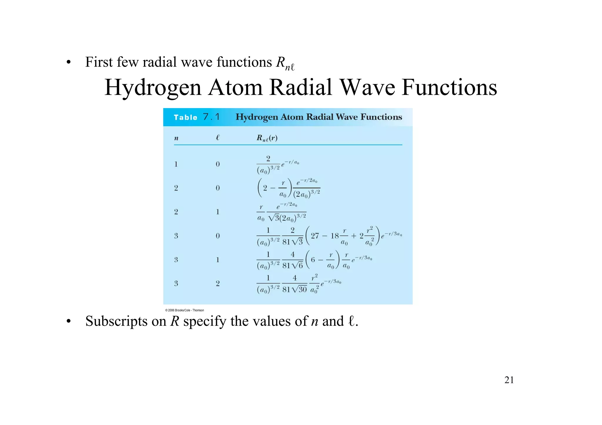
This document summarizes the key steps in solving the time-independent Schrodinger equation for the hydrogen atom using spherical polar coordinates. It separates the equation into three one-dimensional equations for the radial, angular, and azimuthal variables (R(r), Θ(θ), Φ(φ)). Solving each equation shows they are only satisfied for discrete quantum numbers like angular momentum l and principal quantum number n, resulting in quantization of the hydrogen atom's energy levels.