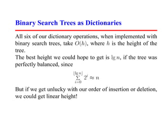
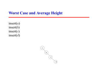
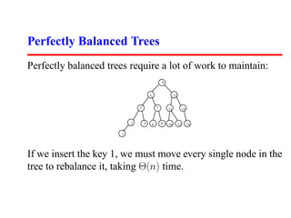
This document discusses dictionaries and binary search trees. It describes the basic operations for dictionaries like search, insert, delete, min, max, successor, and predecessor. It then explains how to implement these operations using binary search trees. The time complexity of each operation is O(h) where h is the height of the tree, which can be O(lg n) for a balanced tree but O(n) in the worst case for an unbalanced tree. Balanced search trees like red-black trees and AVL trees help guarantee O(lg n) time for operations.

1. Lecture 5:
Dictionaries
Steven Skiena
Department of Computer Science
State University of New York
Stony Brook, NY 11794–4400
http://www.cs.sunysb.edu/∼skiena

2. Dictionary / Dynamic Set Operations
Perhaps the most important class of data structures maintain
a set of items, indexed by keys.
• Search(S,k) – A query that, given a set S and a key value
k, returns a pointer x to an element in S such that key[x]
= k, or nil if no such element belongs to S.
• Insert(S,x) – A modifying operation that augments the set
S with the element x.
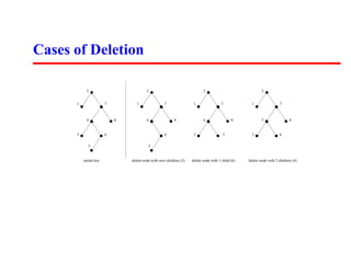
• Delete(S,x) – Given a pointer x to an element in the set S,
remove x from S. Observe we are given a pointer to an
element x, not a key value.

3. • Min(S), Max(S) – Returns the element of the totally
ordered set S which has the smallest (largest) key.
• Next(S,x), Previous(S,x) – Given an element x whose key
is from a totally ordered set S, returns the next largest
(smallest) element in S, or NIL if x is the maximum
(minimum) element.
There are a variety of implementations of these dictionary
operations, each of which yield different time bounds for
various operations.

4. Problem of the Day
What is the asymptotic worst-case running times for each of
the seven fundamental dictionary operations when the data
structure is implemented as
• A singly-linked unsorted list,
• A doubly-linked unsorted list,
• A singly-linked sorted list, and finally
• A doubly-linked sorted list.

5. Solution Blank
singly singly doubly doubly
unsorted sorted unsorted sorted
Search(L, k)
Insert(L, x)
Delete(L, x)
Successor(L, x)
Predecessor(L, x)
Minimum(L)
Maximum(L)

6. Solution
singly double singly doubly
Dictionary operation unsorted unsorted sorted sorted
Search(L, k) O(n) O(n) O(n) O(n)
Insert(L, x) O(1) O(1) O(n) O(n)
Delete(L, x) O(n)∗ O(1) O(n)∗ O(1)
Successor(L, x) O(n) O(n) O(1) O(1)
Predecessor(L, x) O(n) O(n) O(n)∗ O(1)
Minimum(L) O(n) O(n) O(1) O(1)
Maximum(L) O(n) O(n) O(1)∗ O(1)

7. Binary Search Trees
Binary search trees provide a data structure which efficiently
supports all six dictionary operations.
A binary tree is a rooted tree where each node contains at
most two children.
Each child can be identified as either a left or right child.
parent
left right

8. Binary Search Trees
A binary search tree labels each node x in a binary tree such
that all nodes in the left subtree of x have keys < x and all
nodes in the right subtree of x have key’s > x.
2
3
7
6 8
5
The search tree labeling enables us to find where any key is.

9. Implementing Binary Search Trees
typedef struct tree {
item type item;
struct tree *parent;
struct tree *left;
struct tree *right;
} tree;
The parent link is optional, since we can store the pointer on
a stack when we encounter it.

10. Searching in a Binary Tree: Implementation
tree *search tree(tree *l, item type x)
{
if (l == NULL) return(NULL);
if (l->item == x) return(l);
if (x < l->item)
return( search tree(l->left, x) );
else
return( search tree(l->right, x) );
}

11. Searching in a Binary Tree: How Much
The algorithm works because both the left and right subtrees
of a binary search tree are binary search trees – recursive
structure, recursive algorithm.
This takes time proportional to the height of the tree, O(h).

12. Maximum and Minimum
Where are the maximum and minimum elements in a binary
search tree?

13. Finding the Minimum
tree *find minimum(tree *t)
{
tree *min; (* pointer to minimum *)
if (t == NULL) return(NULL);
min = t;
while (min->left != NULL)
min = min->left;
return(min);
}
Finding the max or min takes time proportional to the height
of the tree, O(h).

14. Where is the Predecessor: Internal Node
X
PREDECESSOR(X) SUCCESSOR(X)
If X has two children, its predecessor is the maximum value
in its left subtree and its successor the minimum value in its
right subtree.

15. Where is the Successor: Leaf Node
predecessor(x)
X
If it does not have a left child, a node’s predecessor is its first
left ancestor.
The proof of correctness comes from looking at the in-order
traversal of the tree.

16. In-Order Traversal
void traverse tree(tree *l)
{
if (l != NULL) {
traverse tree(l->left);
process item(l->item);
traverse tree(l->right);
} }
H
A
F
B G
D
C E

17. Tree Insertion
Do a binary search to find where it should be, then replace the
termination NIL pointer with the new item.
1
3
2 7
6 8
5
Insertion takes time proportional to the height of the tree,
O(h).

18. insert tree(tree **l, item type x, tree *parent)
{
tree *p; (* temporary pointer *)
if (*l == NULL) {
p = malloc(sizeof(tree)); (* allocate new node *)
p->item = x;
p->left = p->right = NULL;
p->parent = parent;
*l = p; (* link into parent’s record *)
return;
}
if (x < (*l)->item)
insert tree(&((*l)->left), x, *l);
else
insert tree(&((*l)->right), x, *l);
}

19. Tree Deletion
Deletion is trickier than insertion, because the node to die
may not be a leaf, and thus effect other nodes.
There are three cases:
Case (a), where the node is a leaf, is simple - just NIL out the
parents child pointer.
Case (b), where a node has one chld, the doomed node can
just be cut out.
Case (c), relabel the node as its successor (which has at most
one child when z has two children!) and delete the successor!

20. Cases of Deletion
2 2 2 2
1 7 1 7 1 7 1 7
4 8 4 8 4 8 5 8
3 6 6 3 5 3 6
5 5
initial tree delete node with zero children (3) delete node with 1 child (6) delete node with 2 children (4)

21. Binary Search Trees as Dictionaries
All six of our dictionary operations, when implemented with
binary search trees, take O(h), where h is the height of the
tree.
The best height we could hope to get is lg n, if the tree was
perfectly balanced, since
lg n
2i ≈ n
i=0
But if we get unlucky with our order of insertion or deletion,
we could get linear height!

22. Worst Case and Average Height
insert(a)
insert(b)
insert(c)
insert(d)
A
B
C
D

23. Tree Insertion Analysis
In fact, binary search trees constructed with random insertion
orders on average have Θ(lg n) height.
The worst case is linear, however.
Our analysis of Quicksort will later explain why the expected
height is Θ(lg n).

24. Perfectly Balanced Trees
Perfectly balanced trees require a lot of work to maintain:
9
5 13
3 7 11 15
2 4 6 8 10 12 14
1
If we insert the key 1, we must move every single node in the
tree to rebalance it, taking Θ(n) time.

25. Balanced Search Trees
Therefore, when we talk about ”balanced” trees, we mean
trees whose height is O(lg n), so all dictionary operations
(insert, delete, search, min/max, successor/predecessor) take
O(lg n) time.
Extra care must be taken on insertion and deletion to
guarantee such performance, by rearranging things when they
get too lopsided.
Red-Black trees, AVL trees, 2-3 trees, splay trees, and B-trees
are examples of balanced search trees used in practice and
discussed in most data structure texts.