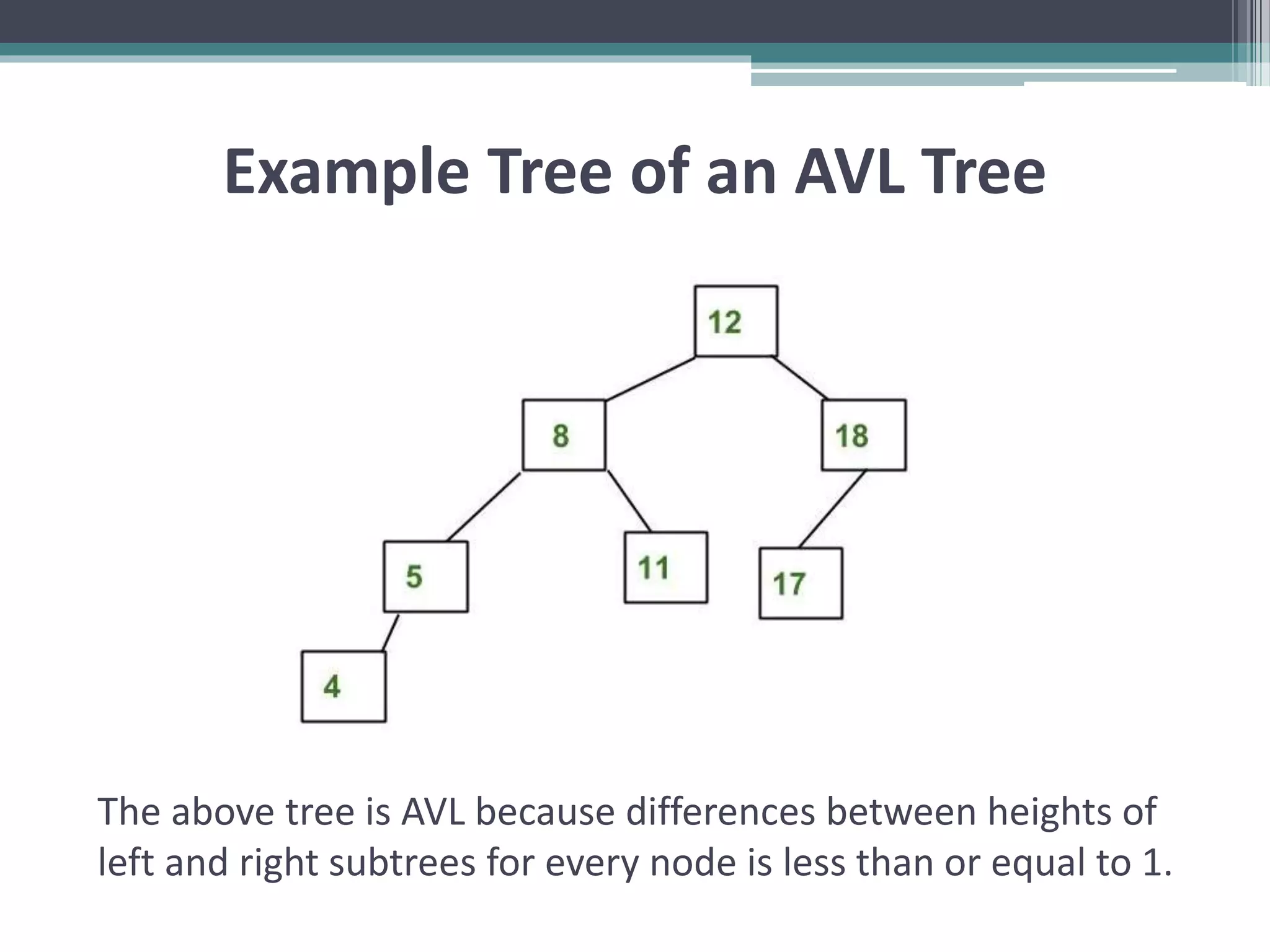
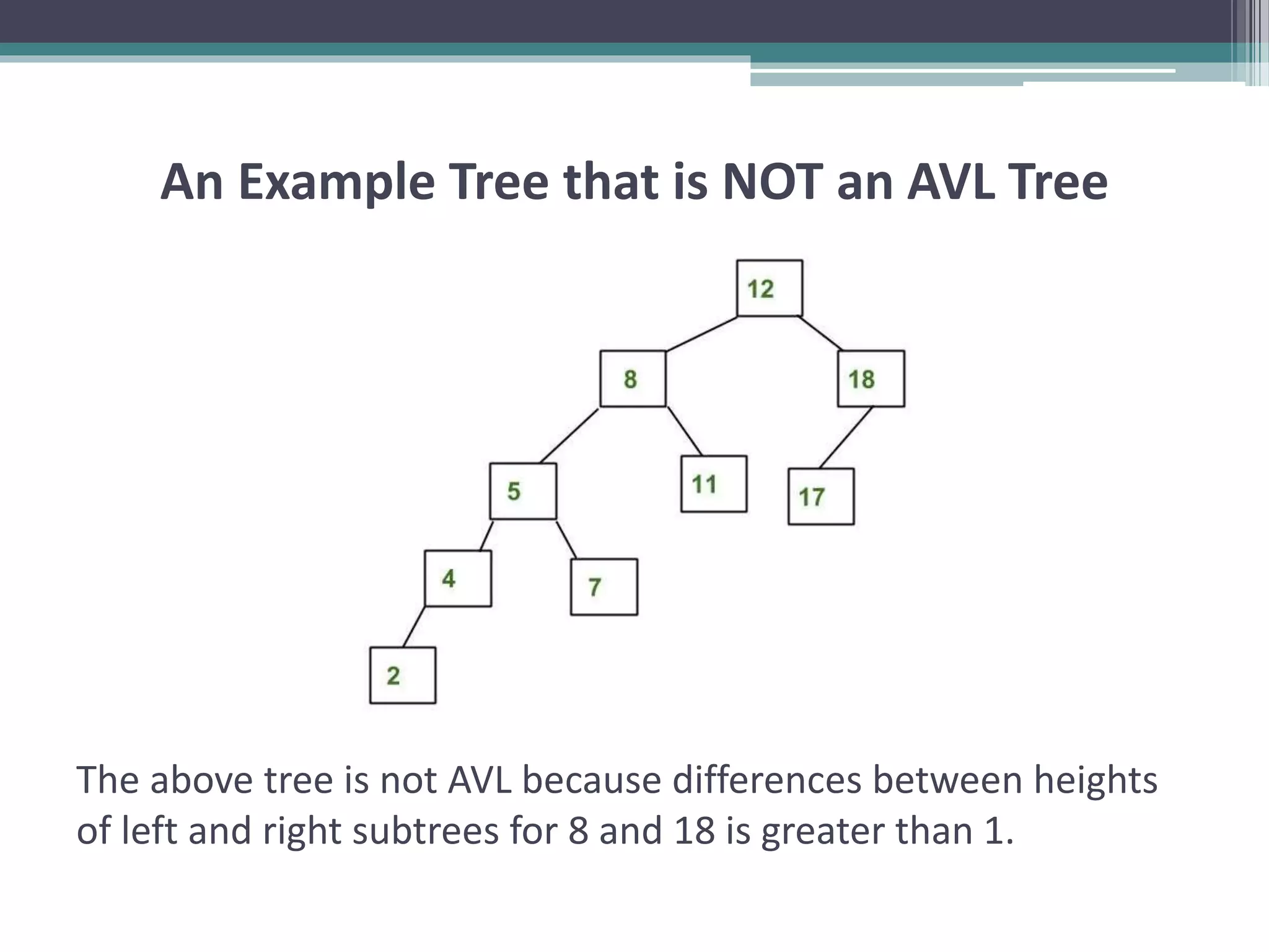
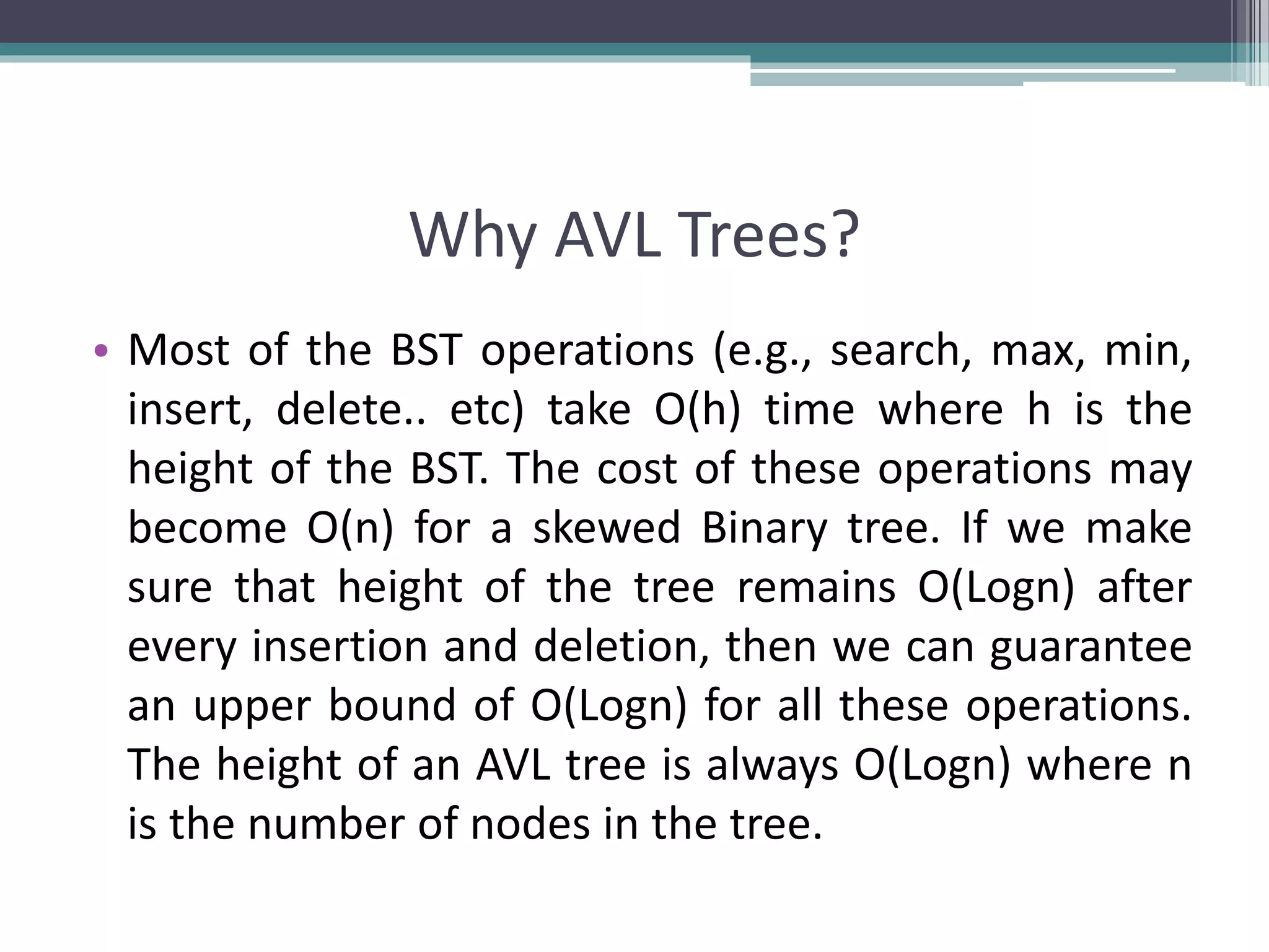
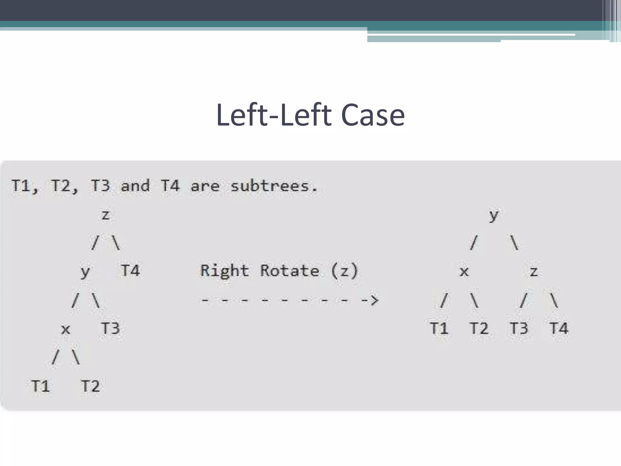
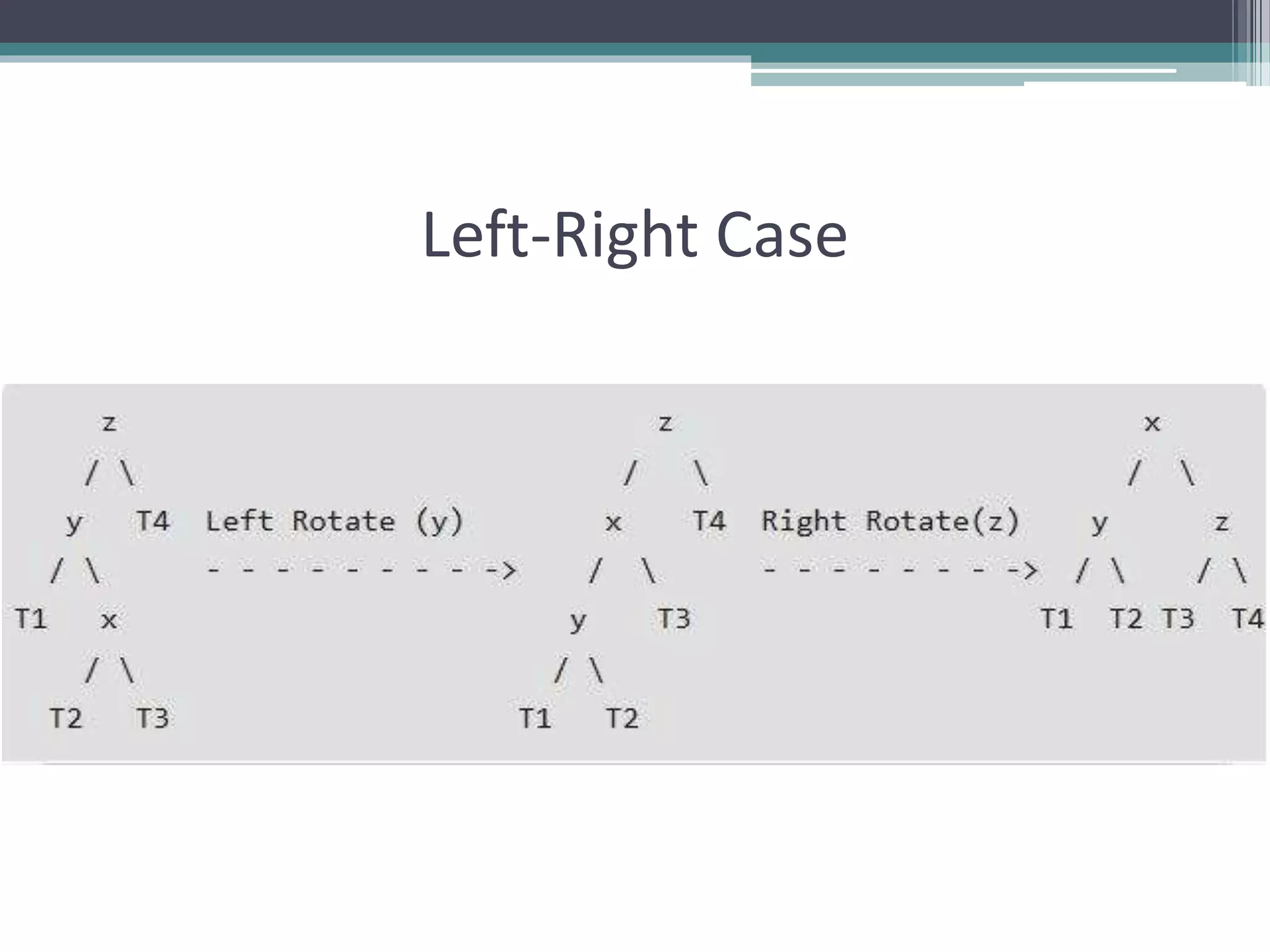
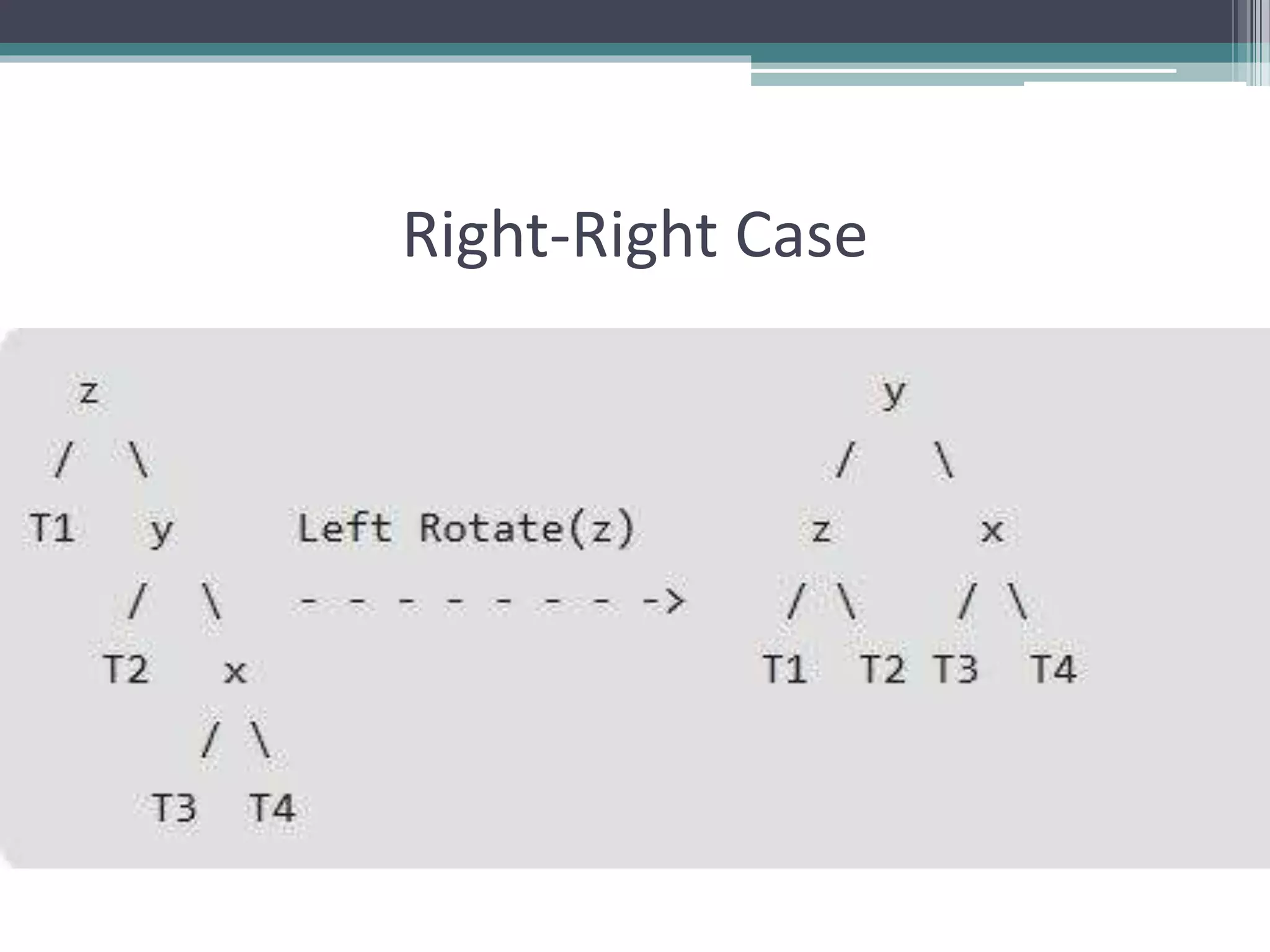
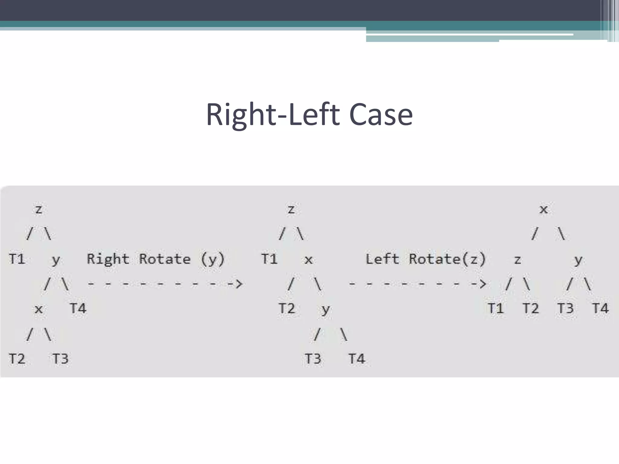
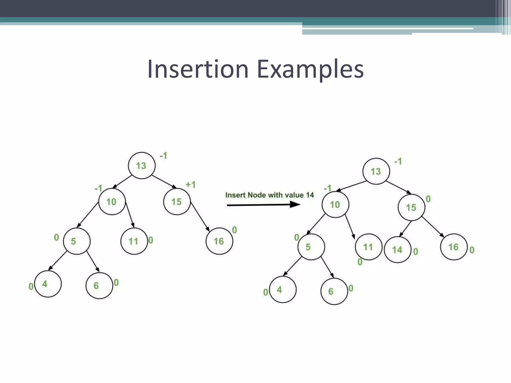
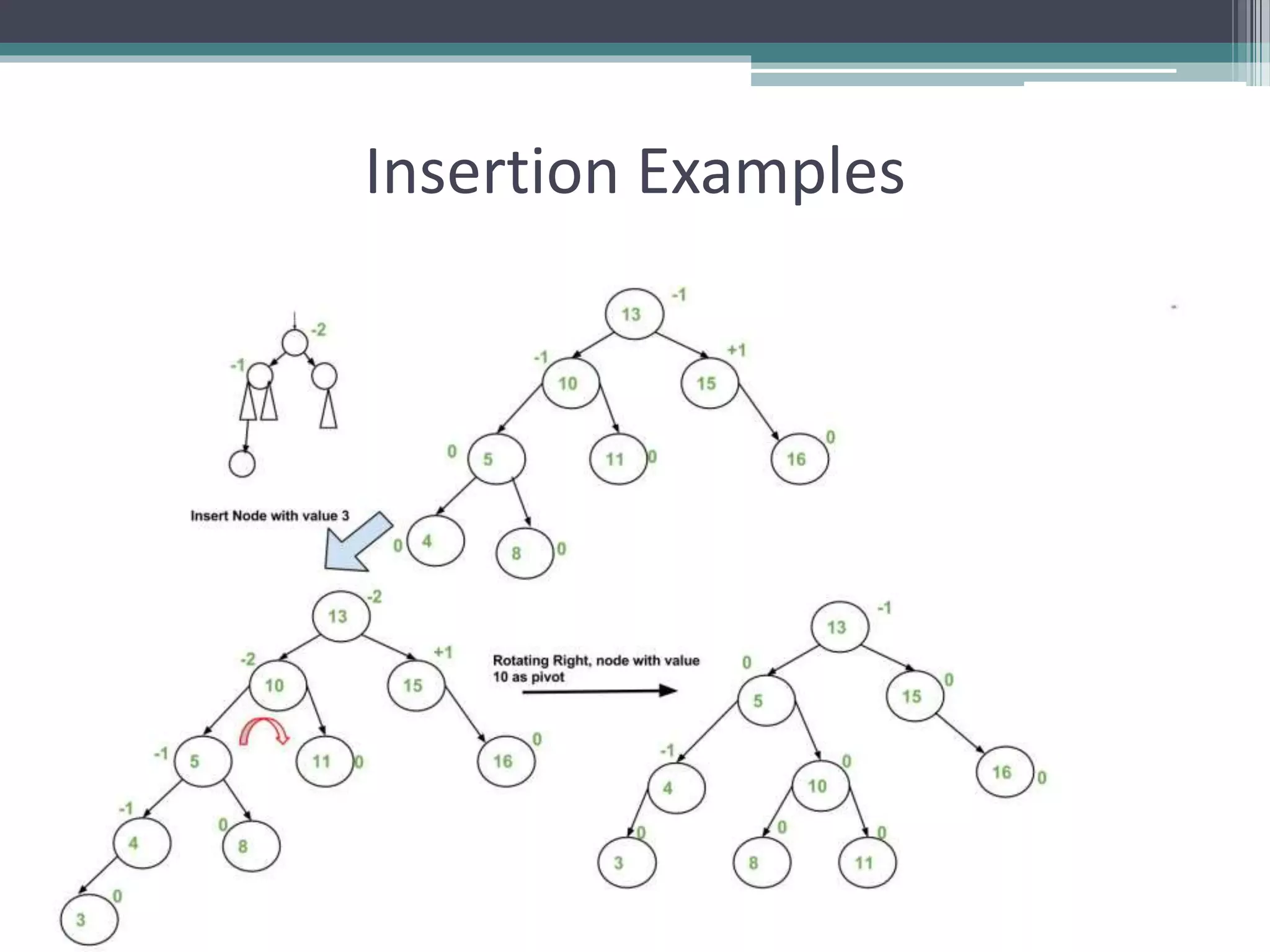
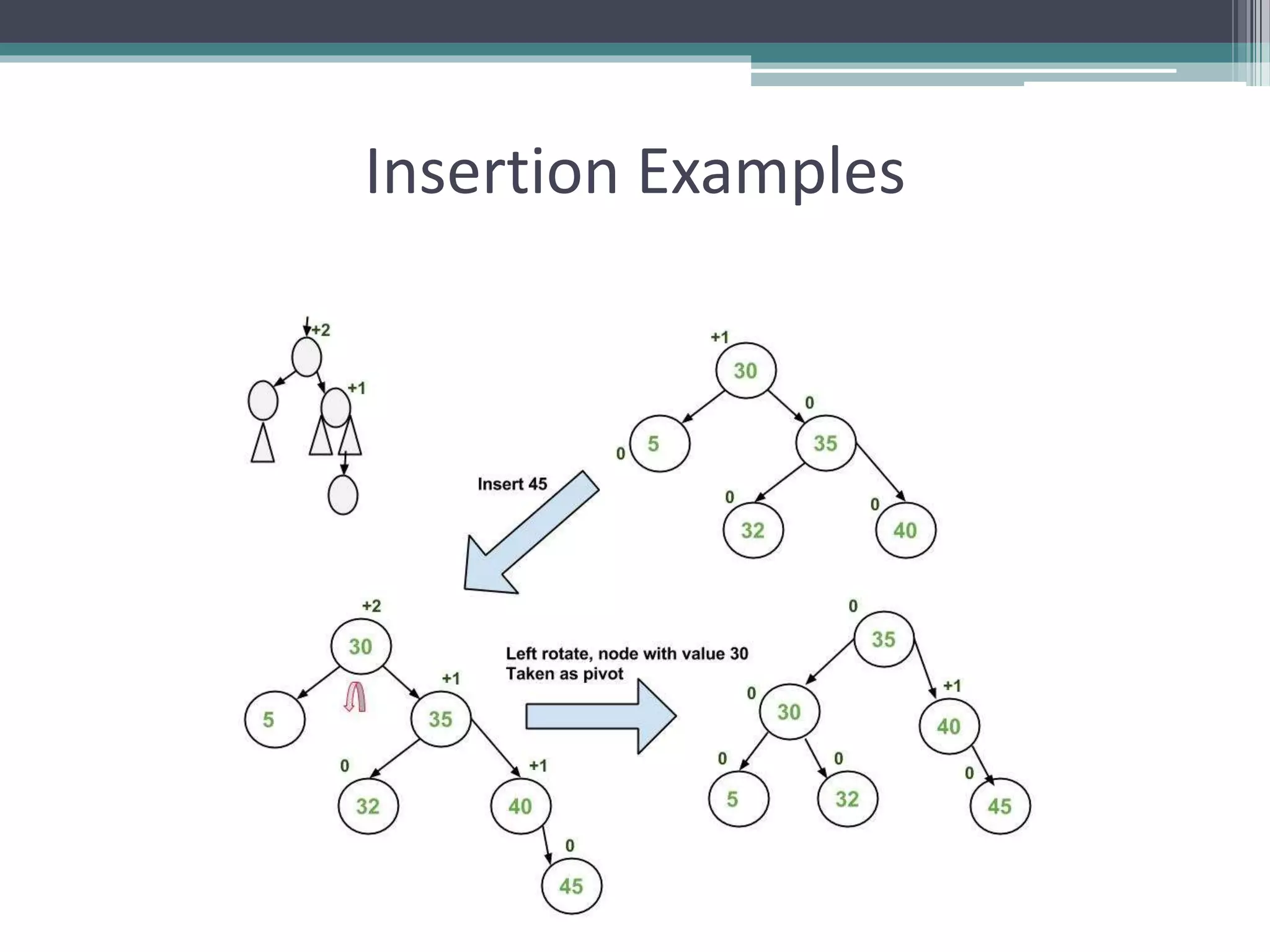
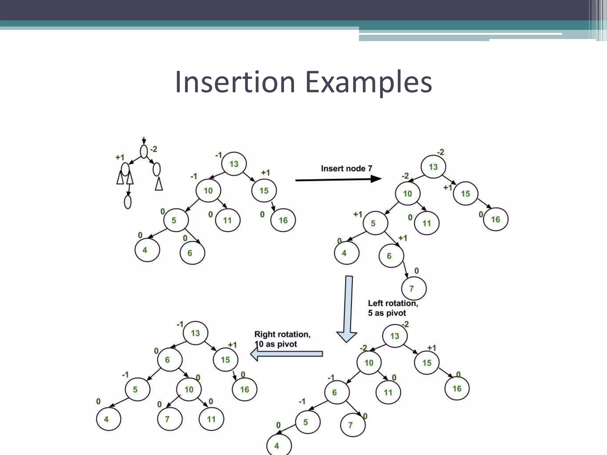
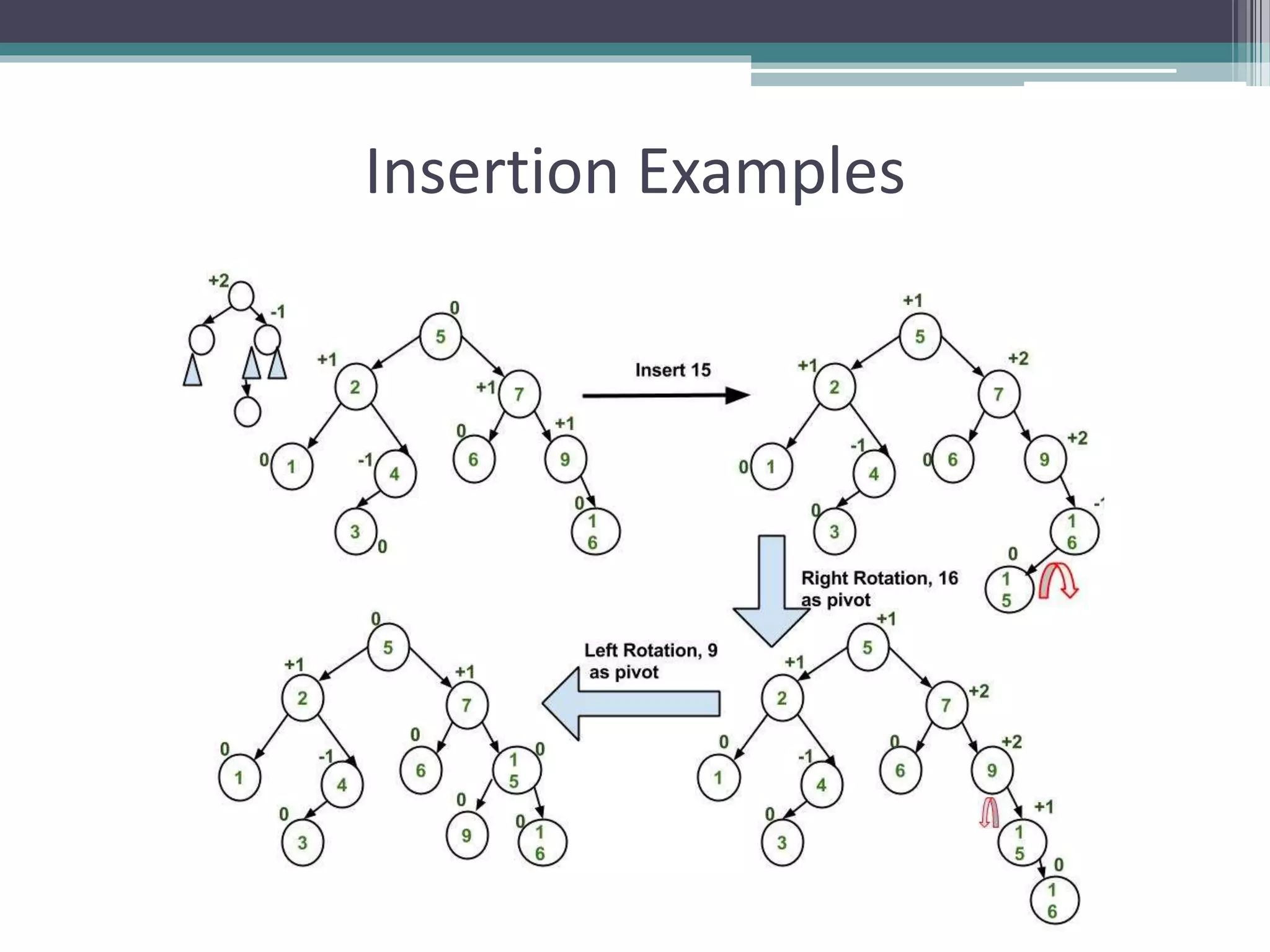
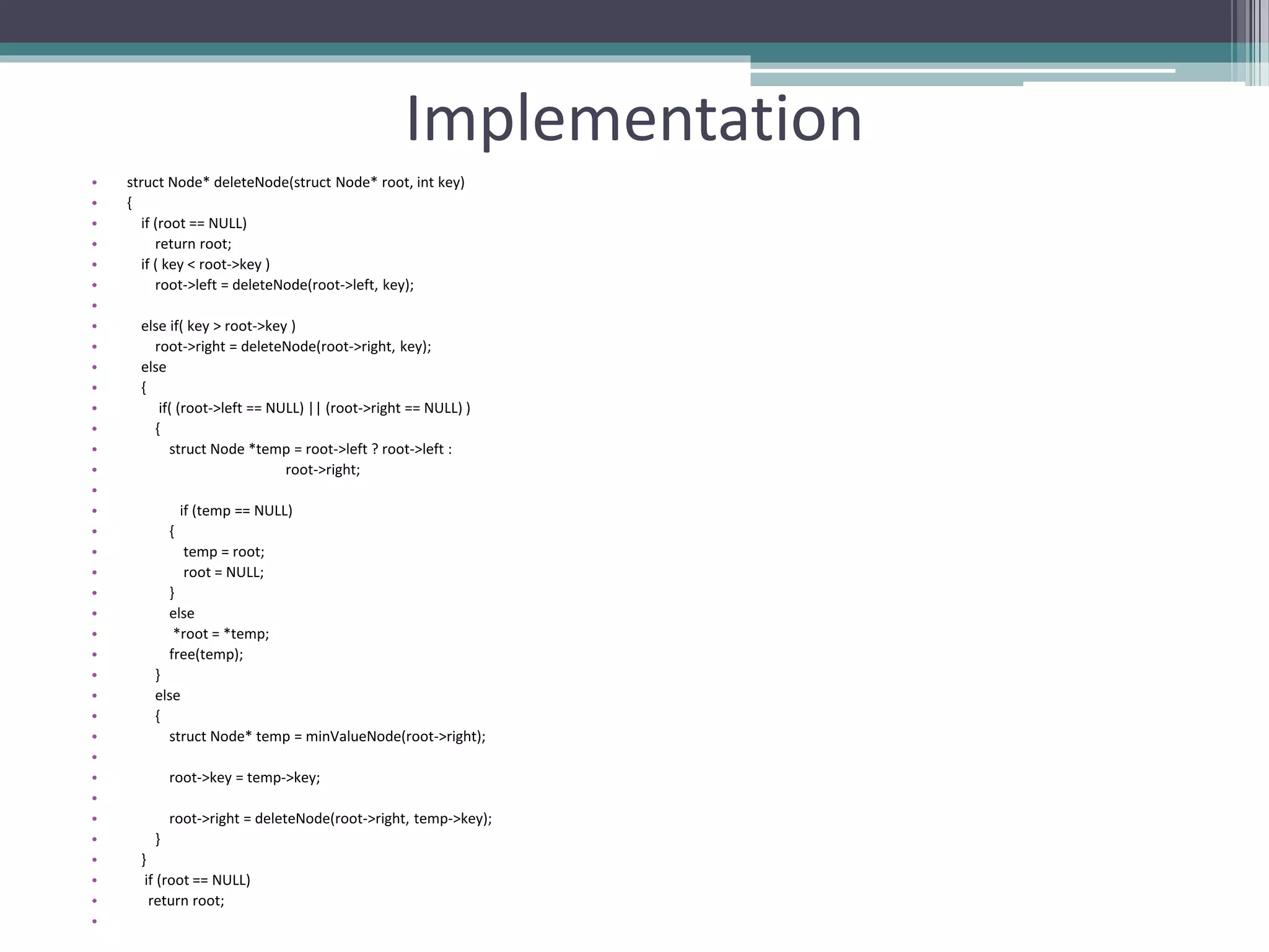
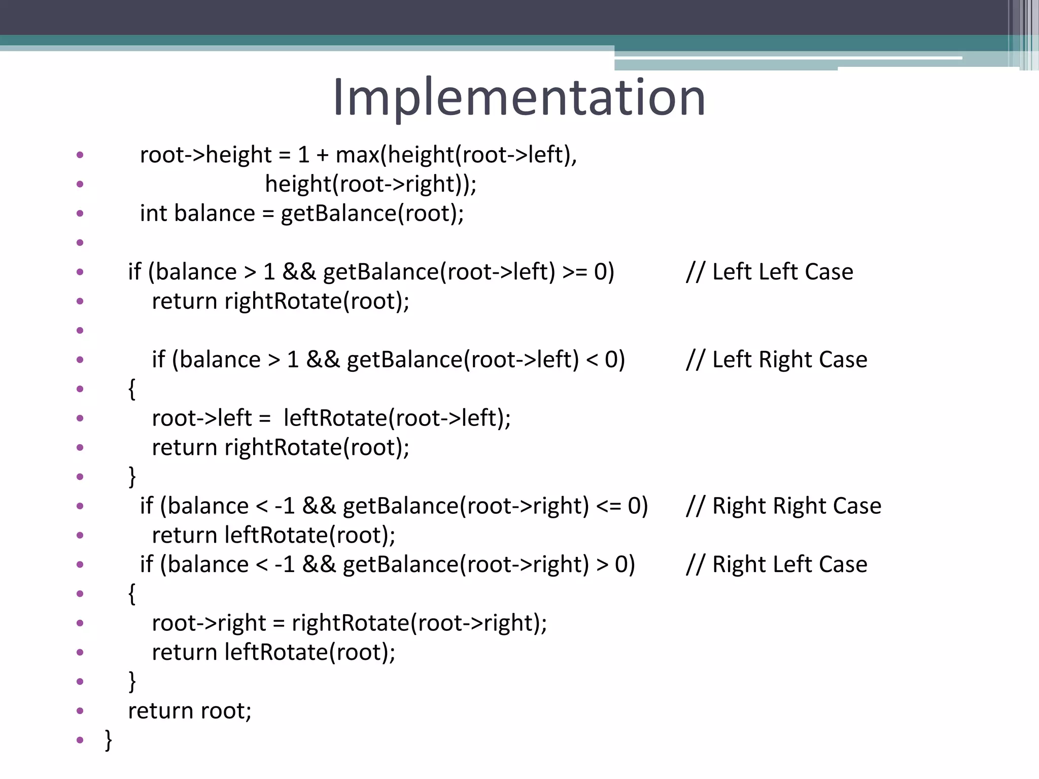
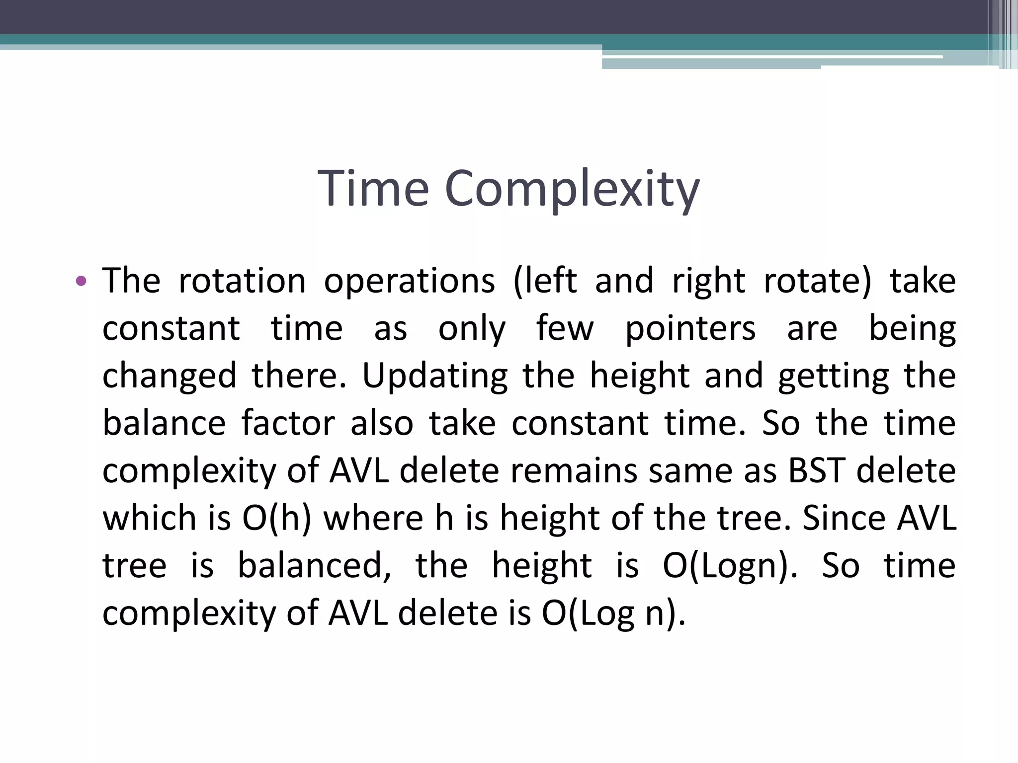
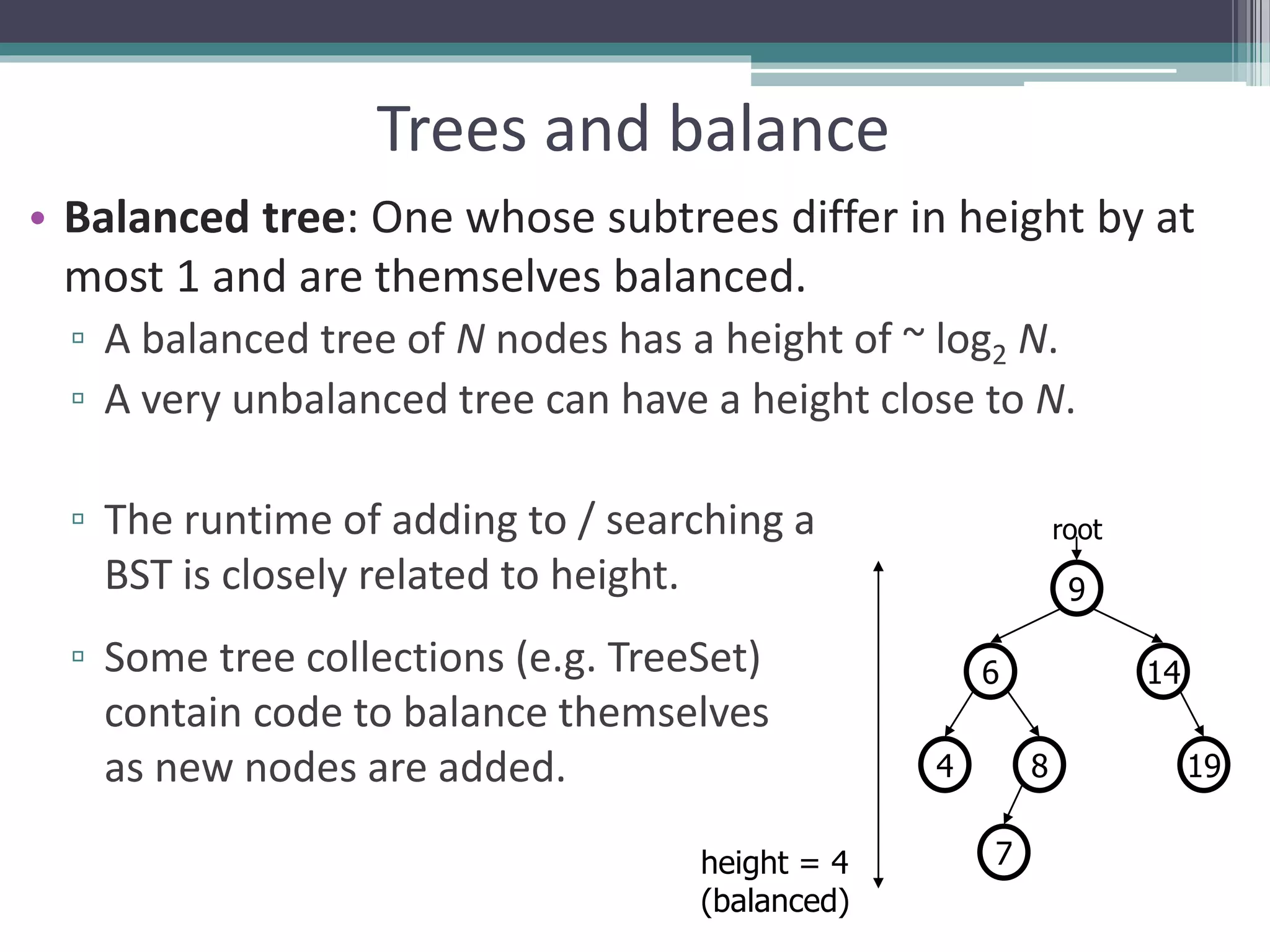
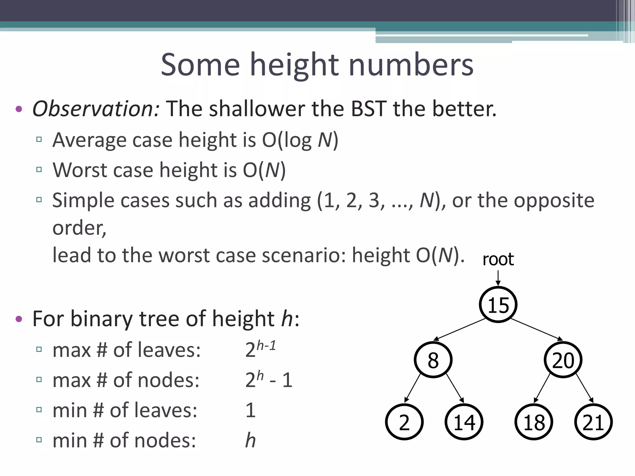
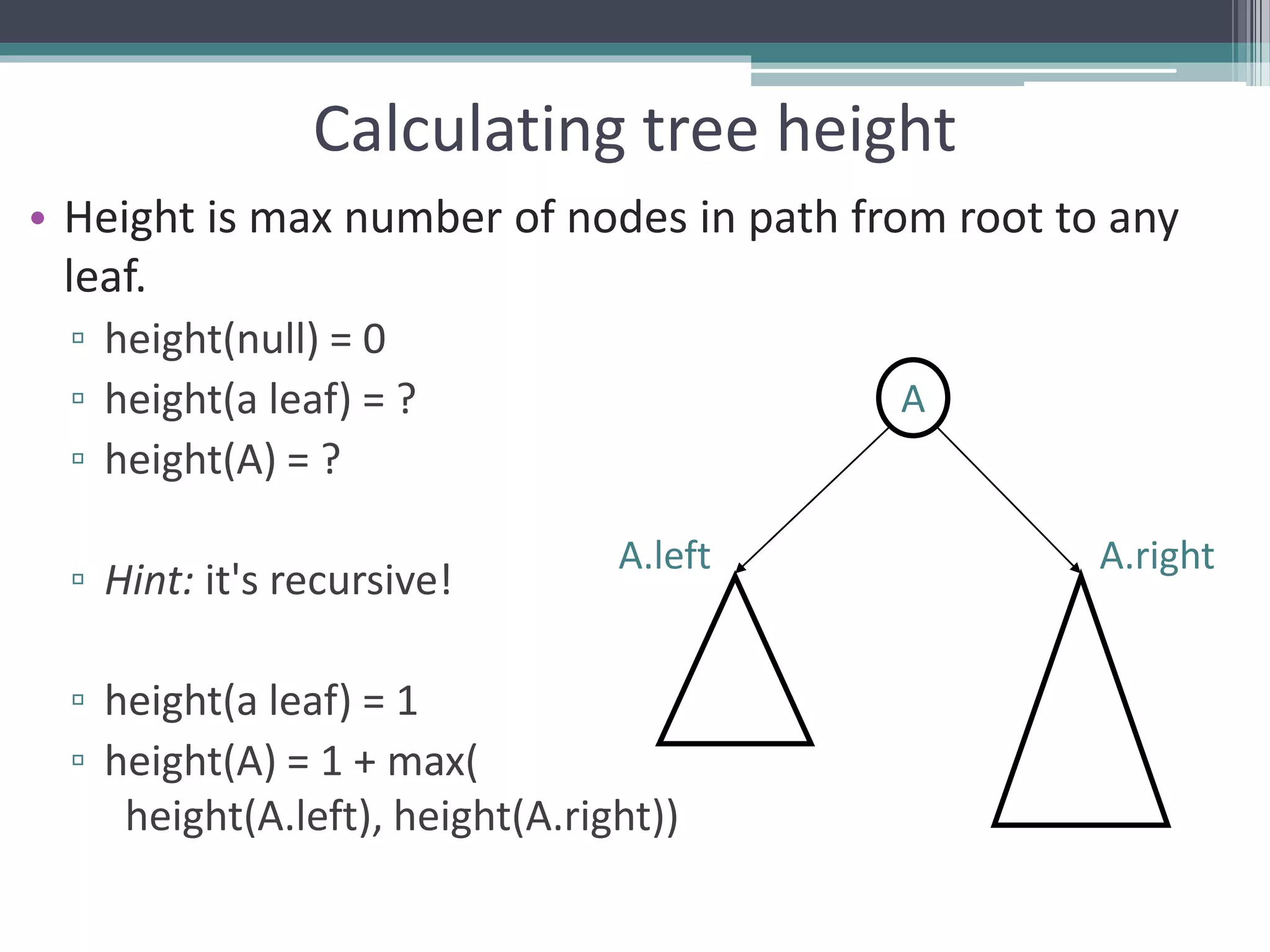
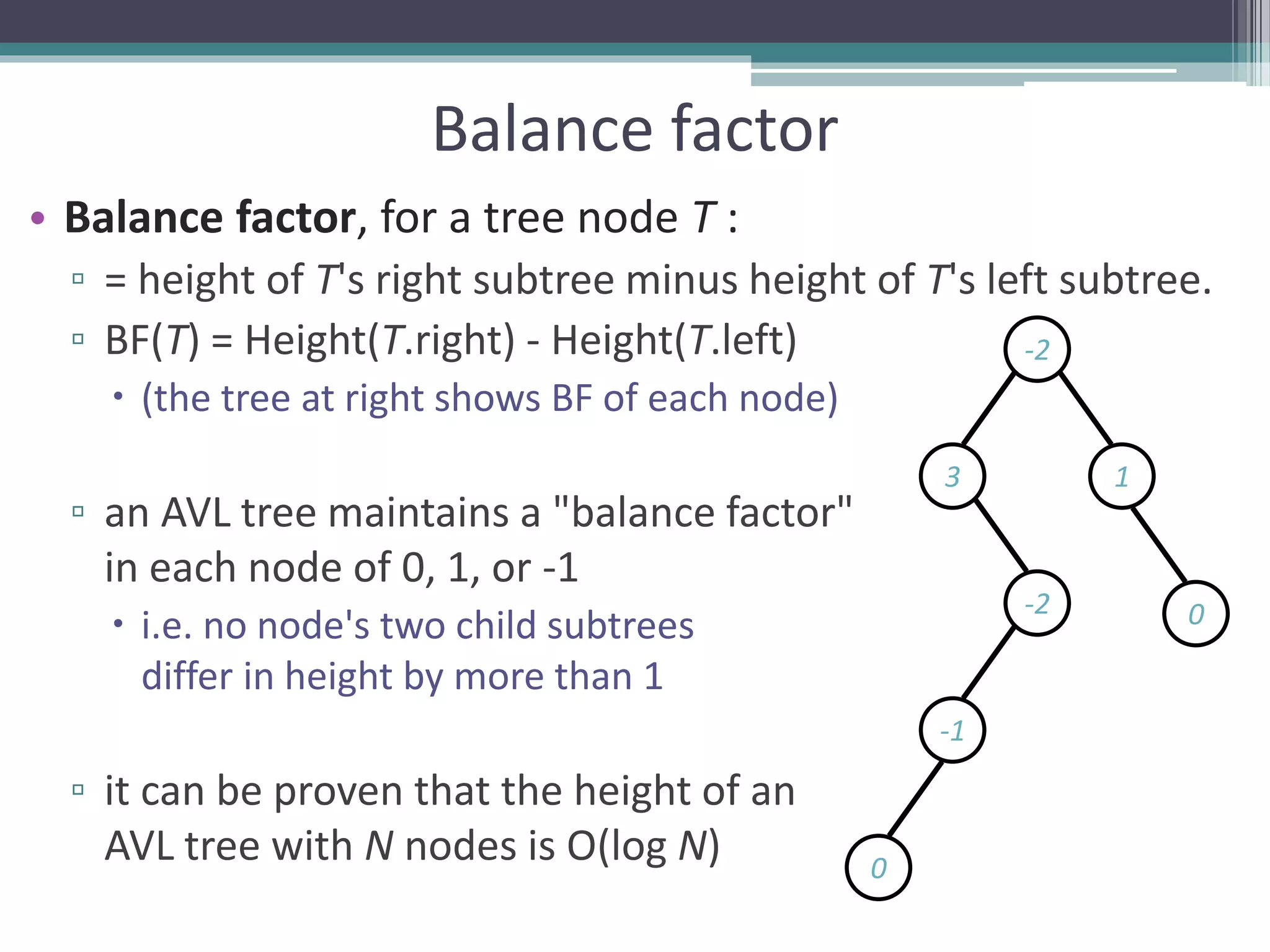
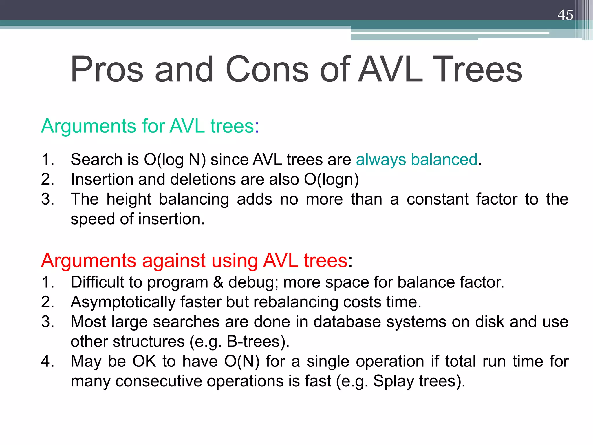
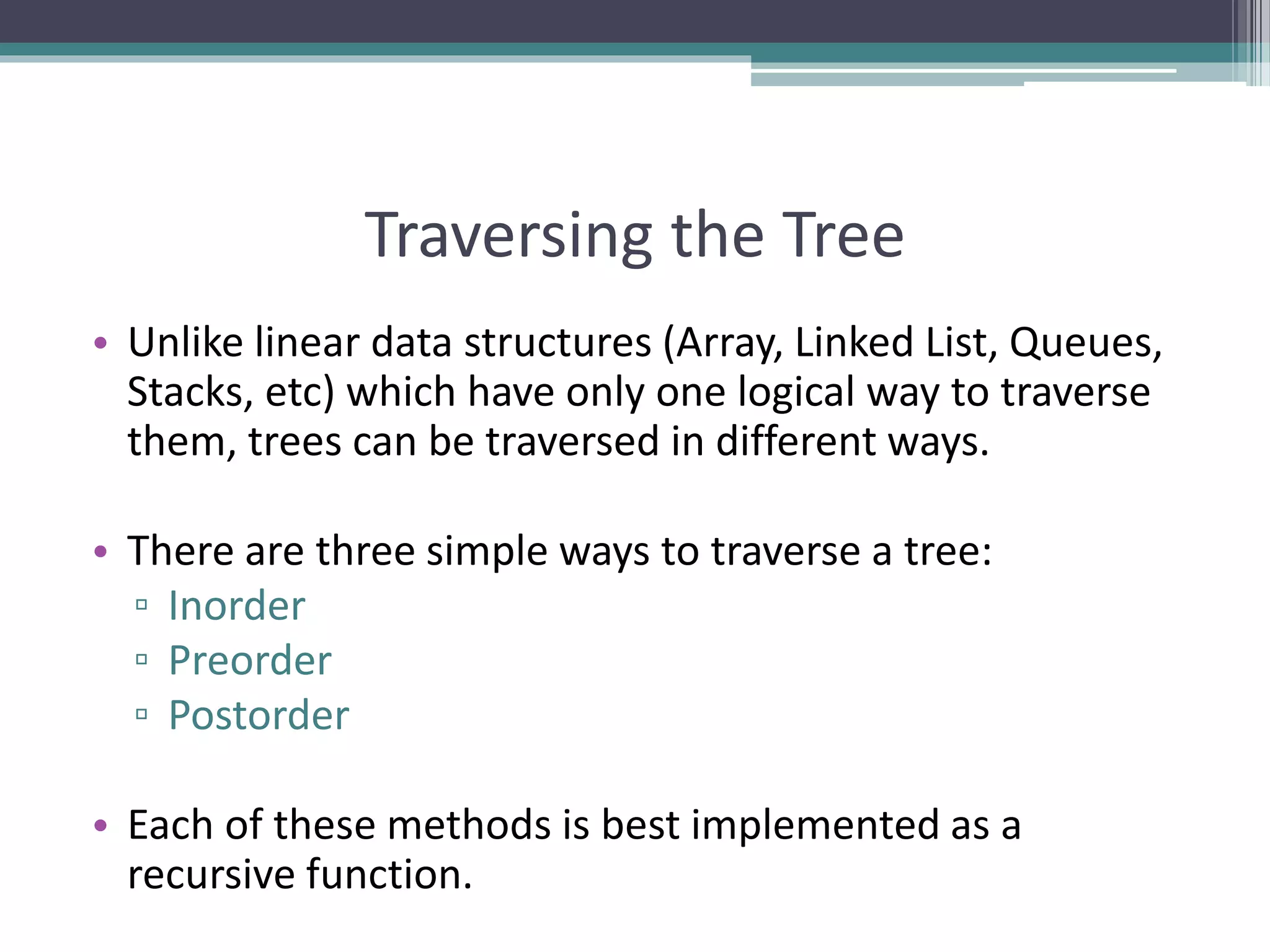
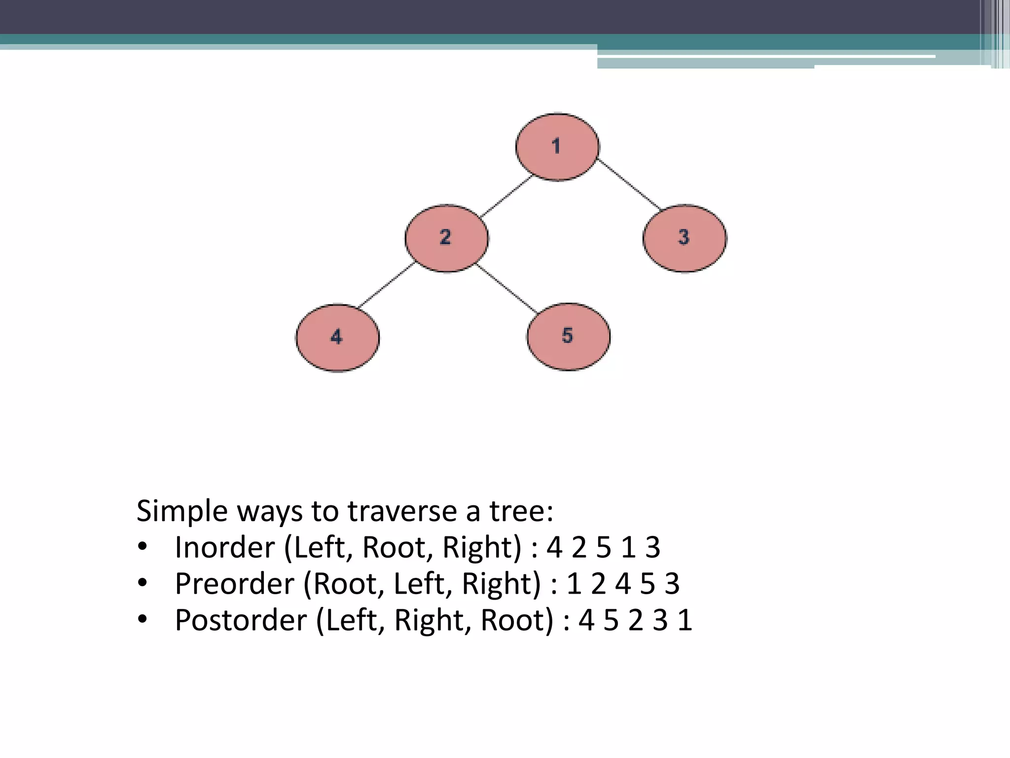
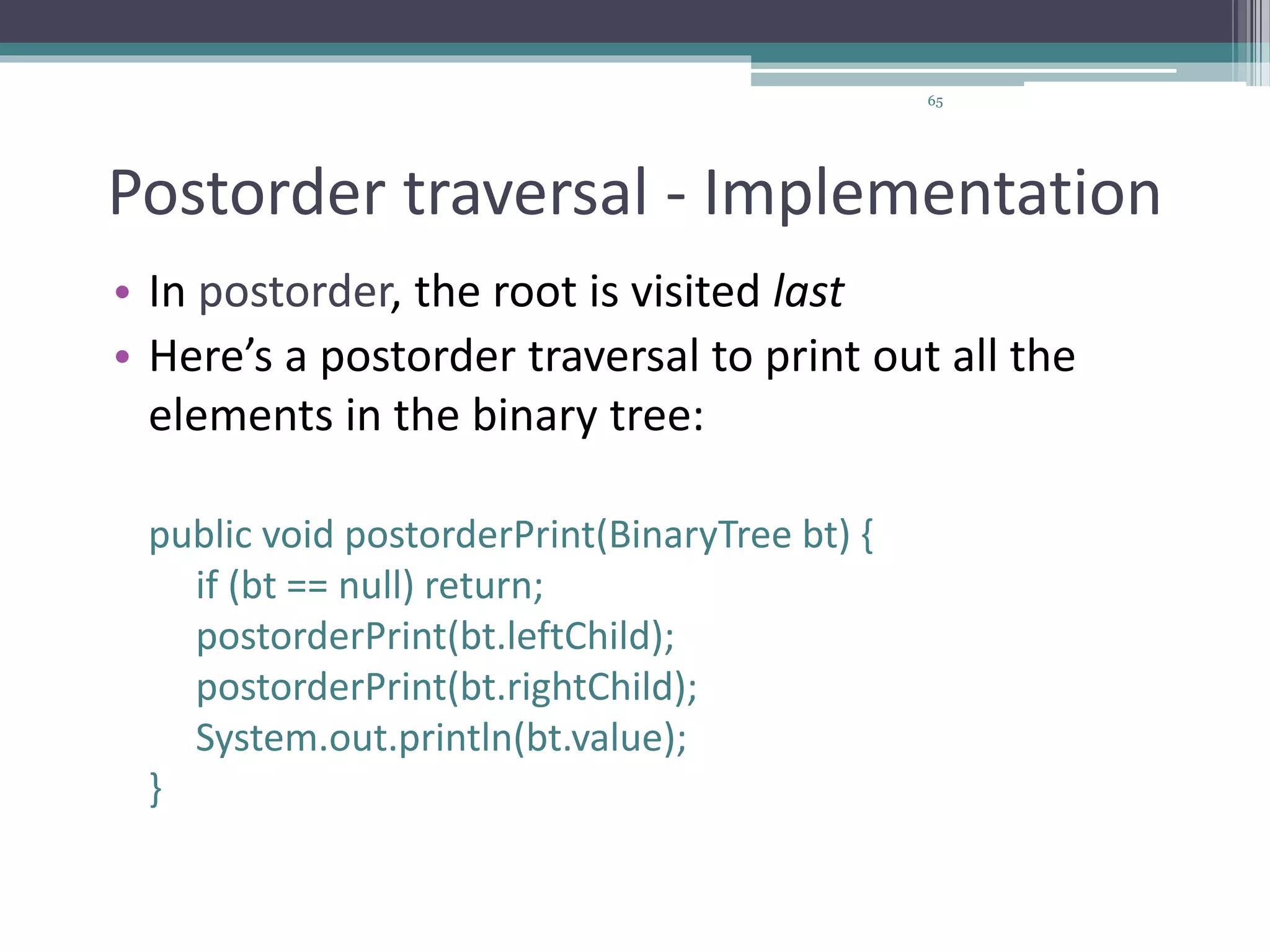
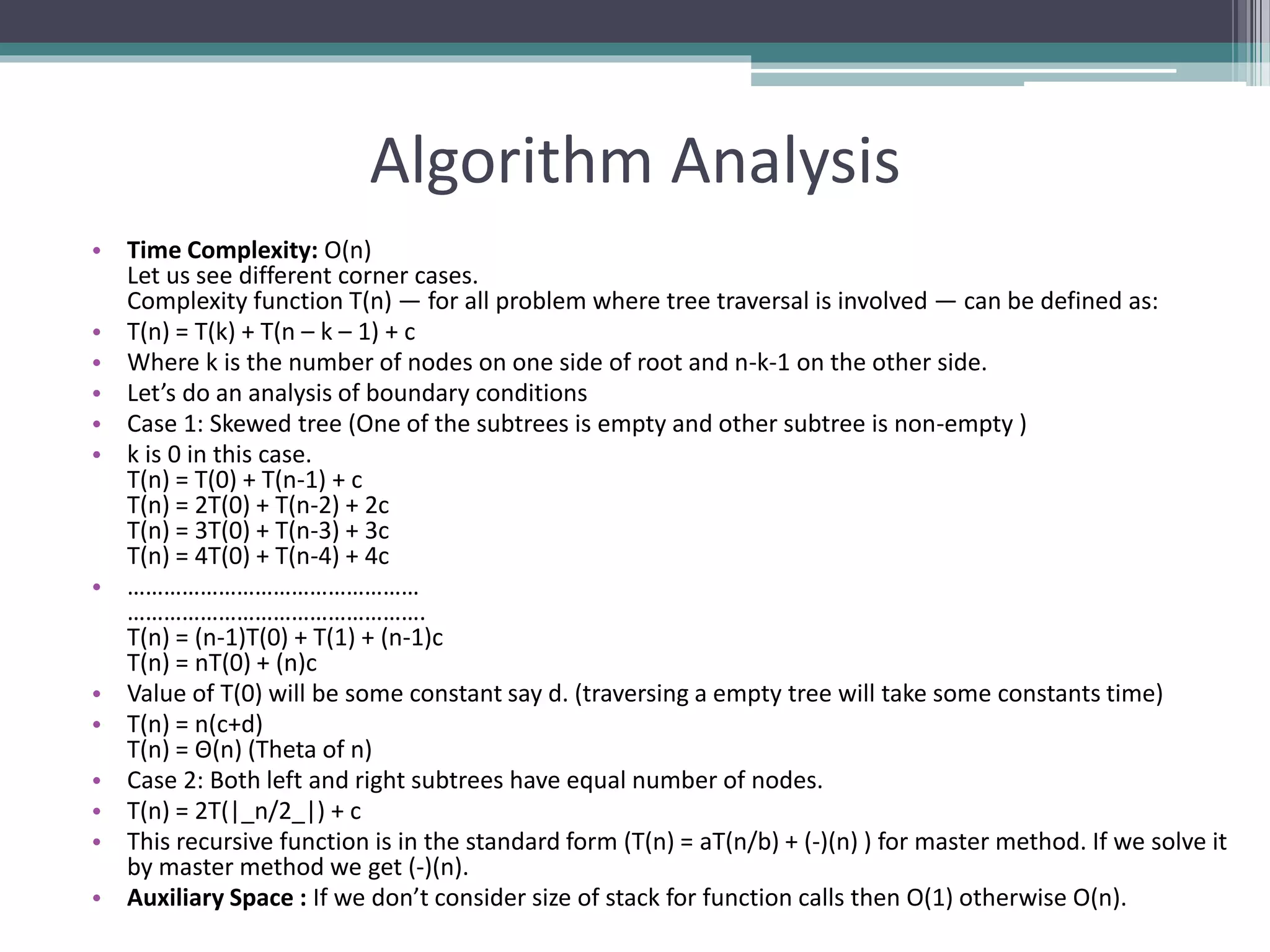
AVL Tree Data Structure

AVL Tree
Prepared by: Afaq Mansoor Khan
BSSE III- Group A
Session 2017-21
IMSciences, Peshawar.

Last Lecture Summary
• Recursive and Non Recursive Traversal of
Binary/Binary Search Tree
• In-Order Traversal
• Pre-Order Traversal
• Post-Order Traversal
• Searching in a Binary Search Tree

Objectives Overview
• Introduction to AVL tree
• Insertion and deletion of a node in AVL tree.
• Balancing of Tree
• Calculating Height of a particular node in the Tree
• Calculating balance Factor for a particular Node in
the Tree
• Left Rotation in an AVL Tree
• Right Rotation in an AVL Tree
• All types of Traversals in AVL
• Algorithm Analysis

Definition of an AVL tree
AVL tree is a self-balancing Binary Search Tree (BST)
where the difference between heights of left and right
subtrees cannot be more than one for all nodes.
It has the following properties:
• The sub-trees of every node differ in height by at
most one.
• Every sub-tree is an AVL tree.

Example Tree of an AVL Tree
The above tree is AVL because differences between heights of
left and right subtrees for every node is less than or equal to 1.

An Example Tree that is NOT an AVL Tree
The above tree is not AVL because differences between heights
of left and right subtrees for 8 and 18 is greater than 1.

Why AVL Trees?
• Most of the BST operations (e.g., search, max, min,
insert, delete.. etc) take O(h) time where h is the
height of the BST. The cost of these operations may
become O(n) for a skewed Binary tree. If we make
sure that height of the tree remains O(Logn) after
every insertion and deletion, then we can guarantee
an upper bound of O(Logn) for all these operations.
The height of an AVL tree is always O(Logn) where n
is the number of nodes in the tree.

Insertion
To make sure that the given tree remains AVL after
every insertion, we must augment the standard BST
insert operation to perform some re-balancing.
Following are two basic operations that can be
performed to re-balance a BST without violating the
BST property (keys(left) < key(root) < keys(right)).
1. Left Rotation
2. Right Rotation

Insertion - Algorithm
Steps:
Let the newly inserted node be w
1. Perform standard BST insert for w.
2. Starting from w, travel up and find the first
unbalanced node. Let z be the first unbalanced
node, y be the child of z that comes on the path
from w to z and x be the grandchild of z that comes
on the path from w to z.
3. Re-balance the tree by performing appropriate
rotations on the subtree rooted with z.

Four Possible Arrangements
There can be 4 possible cases that needs to be handled as x, y
and z can be arranged in 4 ways. Following are the possible 4
arrangements:
a) y is left child of z and x is left child of y (Left-Left Case)
b) y is left child of z and x is right child of y (Left-Right Case)
c) y is right child of z and x is right child of y (Right-Right Case)
d) y is right child of z and x is left child of y (Right-Left Case)

Implementation
This implementation uses the recursive BST insert to insert a new node. In the
recursive BST insert, after insertion, we get pointers to all ancestors one by one in a
bottom-up manner. So we don’t need parent pointer to travel up. The recursive code
itself travels up and visits all the ancestors of the newly inserted node.
1. Perform the normal BST insertion.
2. The current node must be one of the ancestors of the newly inserted node.
Update the height of the current node.
3. Get the balance factor (left subtree height – right subtree height) of the current
node.
4. If balance factor is greater than 1, then the current node is unbalanced and we
are either in Left-Left case or left Right case. To check whether it is left-left case
or not, compare the newly inserted key with the key in left subtree root.
5. If balance factor is less than -1, then the current node is unbalanced and we are
either in Right-Right case or Right-Left case. To check whether it is Right-Right
case or not, compare the newly inserted key with the key in right subtree root.

Implementation
• struct Node* insert(struct Node* node, int key)
• {
• if (node == NULL)
• return(newNode(key));
•
• if (key < node->key)
• node->left = insert(node->left, key);
• else if (key > node->key)
• node->right = insert(node->right, key);
• else return node;
• node->height = 1 + max(height(node->left),
• height(node->right));
• int balance = getBalance(node);
•
• if (balance > 1 && key < node->left->key) // Left Left Case
• return rightRotate(node);
•
• if (balance < -1 && key > node->right->key) // Right Right Case
• return leftRotate(node);
•
• if (balance > 1 && key > node->left->key) // Left Right Case
• {
• node->left = leftRotate(node->left);
• return rightRotate(node);
• }
• if (balance < -1 && key < node->right->key) // Right Left Case
• {
• node->right = rightRotate(node->right);
• return leftRotate(node);
• }
• return node;
• }

Time Complexity
• The rotation operations (left and right rotate) take
constant time as only a few pointers are being
changed there. Updating the height and getting the
balance factor also takes constant time. So the time
complexity of AVL insert remains same as BST insert
which is O(h) where h is the height of the tree. Since
AVL tree is balanced, the height is O(Logn). So time
complexity of AVL insert is O(Logn).

Deletion
To make sure that the given tree remains AVL after
every deletion, we must augment the standard BST
delete operation to perform some re-balancing.
Following are two basic operations that can be
performed to re-balance a BST without violating the
BST property (keys(left) < key(root) < keys(right)).
1. Left Rotation
2. Right Rotation

Deletion - Algorithm
Steps:
Let w be the node to be deleted
1. Perform standard BST delete for w.
2. Starting from w, travel up and find the first
unbalanced node. Let z be the first unbalanced
node, y be the larger height child of z, and x be the
larger height child of y. Note that the definitions of
x and y are different from insertion here.
3. Re-balance the tree by performing appropriate
rotations on the subtree rooted with z.

Four Possible Arrangements
There can be 4 possible cases that needs to be handled as
x, y and z can be arranged in 4 ways. Following are the
possible 4 arrangements:
a) y is left child of z and x is left child of y
(Left-Left Case)
b) y is left child of z and x is right child of y
(Left-Right Case)
c) y is right child of z and x is right child of y
(Right-Right Case)
d) y is right child of z and x is left child of y
(Right-Left Case)

Implementation
The following implementation uses the recursive BST delete as basis. In the
recursive BST delete, after deletion, we get pointers to all ancestors one by
one in bottom up manner. So we don’t need parent pointer to travel up. The
recursive code itself travels up and visits all the ancestors of the deleted
node.
Perform the normal BST deletion.
1. The current node must be one of the ancestors of the deleted node.
Update the height of the current node.
2. Get the balance factor (left subtree height – right subtree height) of the
current node.
3. If balance factor is greater than 1, then the current node is unbalanced
and we are either in Left Left case or Left Right case. To check whether
it is Left Left case or Left Right case, get the balance factor of left
subtree. If balance factor of the left subtree is greater than or equal to
0, then it is Left Left case, else Left Right case.
4. If balance factor is less than -1, then the current node is unbalanced
and we are either in Right Right case or Right Left case. To check
whether it is Right Right case or Right Left case, get the balance factor
of right subtree. If the balance factor of the right subtree is smaller than
or equal to 0, then it is Right Right case, else Right Left case.

Implementation
• struct Node* deleteNode(struct Node* root, int key)
• {
• if (root == NULL)
• return root;
• if ( key < root->key )
• root->left = deleteNode(root->left, key);
•
• else if( key > root->key )
• root->right = deleteNode(root->right, key);
• else
• {
• if( (root->left == NULL) || (root->right == NULL) )
• {
• struct Node *temp = root->left ? root->left :
• root->right;
•
• if (temp == NULL)
• {
• temp = root;
• root = NULL;
• }
• else
• *root = *temp;
• free(temp);
• }
• else
• {
• struct Node* temp = minValueNode(root->right);
•
• root->key = temp->key;
•
• root->right = deleteNode(root->right, temp->key);
• }
• }
• if (root == NULL)
• return root;
•

Implementation
• root->height = 1 + max(height(root->left),
• height(root->right));
• int balance = getBalance(root);
•
• if (balance > 1 && getBalance(root->left) >= 0) // Left Left Case
• return rightRotate(root);
•
• if (balance > 1 && getBalance(root->left) < 0) // Left Right Case
• {
• root->left = leftRotate(root->left);
• return rightRotate(root);
• }
• if (balance < -1 && getBalance(root->right) <= 0) // Right Right Case
• return leftRotate(root);
• if (balance < -1 && getBalance(root->right) > 0) // Right Left Case
• {
• root->right = rightRotate(root->right);
• return leftRotate(root);
• }
• return root;
• }

Time Complexity
• The rotation operations (left and right rotate) take
constant time as only few pointers are being
changed there. Updating the height and getting the
balance factor also take constant time. So the time
complexity of AVL delete remains same as BST delete
which is O(h) where h is height of the tree. Since AVL
tree is balanced, the height is O(Logn). So time
complexity of AVL delete is O(Log n).

Trees and balance
• Balanced tree: One whose subtrees differ in height by at
most 1 and are themselves balanced.
▫ A balanced tree of N nodes has a height of ~ log2 N.
▫ A very unbalanced tree can have a height close to N.
▫ The runtime of adding to / searching a
BST is closely related to height.
▫ Some tree collections (e.g. TreeSet)
contain code to balance themselves
as new nodes are added. 19
7
146
9
84
root
height = 4
(balanced)

Some height numbers
• Observation: The shallower the BST the better.
▫ Average case height is O(log N)
▫ Worst case height is O(N)
▫ Simple cases such as adding (1, 2, 3, ..., N), or the opposite
order,
lead to the worst case scenario: height O(N).
• For binary tree of height h:
▫ max # of leaves: 2h-1
▫ max # of nodes: 2h - 1
▫ min # of leaves: 1
▫ min # of nodes: h
2118
208
15
142
root

Calculating tree height
• Height is max number of nodes in path from root to any
leaf.
▫ height(null) = 0
▫ height(a leaf) = ?
▫ height(A) = ?
▫ Hint: it's recursive!
▫ height(a leaf) = 1
▫ height(A) = 1 + max(
height(A.left), height(A.right))
A
A.left A.right

Balance factor
• Balance factor, for a tree node T :
▫ = height of T's right subtree minus height of T's left subtree.
▫ BF(T) = Height(T.right) - Height(T.left)
 (the tree at right shows BF of each node)
▫ an AVL tree maintains a "balance factor"
in each node of 0, 1, or -1
 i.e. no node's two child subtrees
differ in height by more than 1
▫ it can be proven that the height of an
AVL tree with N nodes is O(log N)
-2
3 1
-1
-2
0
0

45
Arguments for AVL trees:
1. Search is O(log N) since AVL trees are always balanced.
2. Insertion and deletions are also O(logn)
3. The height balancing adds no more than a constant factor to the
speed of insertion.
Arguments against using AVL trees:
1. Difficult to program & debug; more space for balance factor.
2. Asymptotically faster but rebalancing costs time.
3. Most large searches are done in database systems on disk and use
other structures (e.g. B-trees).
4. May be OK to have O(N) for a single operation if total run time for
many consecutive operations is fast (e.g. Splay trees).
Pros and Cons of AVL Trees

Traversing the Tree
• Unlike linear data structures (Array, Linked List, Queues,
Stacks, etc) which have only one logical way to traverse
them, trees can be traversed in different ways.
• There are three simple ways to traverse a tree:
▫ Inorder
▫ Preorder
▫ Postorder
• Each of these methods is best implemented as a
recursive function.

Simple ways to traverse a tree:
• Inorder (Left, Root, Right) : 4 2 5 1 3
• Preorder (Root, Left, Right) : 1 2 4 5 3
• Postorder (Left, Right, Root) : 4 5 2 3 1

Inorder Traversing using Recursion
Inorder traversal will cause all the nodes to be visited in
ascending order.
Steps involved in Inorder traversal (recursion) are:
1. -- Call itself to traverse the node’s left subtree
2. -- Visit the node (e.g. display a key)
3. -- Call itself to traverse the node’s right subtree.

51
Inorder Traversal
1. The node’s left subtree is traversed.
2. The node’s data is processed.
3. The node’s right subtree is traversed.

52
Inorder Traversing - Algorithm
1. Traverse the left subtree, i.e., call Inorder(left-
subtree)
2. Visit the root.
3. Traverse the right subtree, i.e., call
Inorder(right-subtree)

53
Inorder Traversing - Implementation
• In inorder, the root is visited in the middle
• Here’s an inorder traversal to print out all the
elements in the binary tree:
public void inorderPrint(BinaryTree bt) {
if (bt == null) return;
inorderPrint(bt.leftChild);
System.out.println(bt.value);
inorderPrint(bt.rightChild);
}

Non Recursive Inorder Traversing
1) Create an empty stack S.
2) Initialize current node as root
3) Push the current node to S and set current = current->left
until current is NULL
4) If current is NULL and stack is not empty then:
a) Pop the top item from stack.
b) Print the popped item, set current = popped_item->right
c) Go to step 3.
5) If current is NULL and stack is empty then we are done.

Preorder Traversing using Recursion
• Sequence of preorder traversal: e.g. use for infix
parse tree to generate prefix
• Steps involved in Preorder traversal (recursion) are:
-- Visit the node
-- Call itself to traverse the node’s left subtree
-- Call itself to traverse the node’s right subtree

57
Preorder Traversal

58
Preorder Traversing - Algorithm
1. Visit the root.
2. Traverse the left subtree, i.e., call
Preorder(left-subtree)
Preorder(right-subtree)

59
Preorder Traversing - Implementation
• In preorder, the root is visited first
• Here’s a preorder traversal to print out all the
public void preorderPrint(BinaryTree bt) {
preorderPrint(bt.leftChild);
preorderPrint(bt.rightChild);
}

60
Non Recursive Preorder Traversing
• Create a Stack.
• Print the root and push it to Stack and go left
i.e root=root.left and till it hits the NULL.
• If root is null and Stack is empty then
▫ return, we are done.
• Else
▫ Pop the top Node from the Stack and set it as, root
= popped_Node.
▫ Go right, root = root.right.
▫ Go to step 2.
• End If

Postorder Traversing using Recursion
• Sequence of postorder traversal: e.g. use for infix
parse tree to generate postfix
• Steps involved in Postorder traversal (recursion) are:
-- Call itself to traverse the node’s left subtree
-- Call itself to traverse the node’s right subtree
-- Visit the node.

63
Postorder Traversal

64
Postorder traversal - Algorithm
1. Traverse the left subtree, i.e., call
Postorder(left-subtree)
Postorder(right-subtree)
3. Visit the root.

65
Postorder traversal - Implementation
• In postorder, the root is visited last
• Here’s a postorder traversal to print out all the
public void postorderPrint(BinaryTree bt) {
postorderPrint(bt.leftChild);
postorderPrint(bt.rightChild);
}

66
Non Recursive Preorder Traversing
• Push root into Stack_One.
• while(Stack_One is not empty)
▫ Pop the node from Stack_One and push it into
Stack_Two.
▫ Push the left and right child nodes of popped node
into Stack_One.
• End Loop
• Pop out all the nodes from Stack_Two and print
it.

Algorithm Analysis
• Time Complexity: O(n)
Let us see different corner cases.
Complexity function T(n) — for all problem where tree traversal is involved — can be defined as:
• T(n) = T(k) + T(n – k – 1) + c
• Where k is the number of nodes on one side of root and n-k-1 on the other side.
• Let’s do an analysis of boundary conditions
• Case 1: Skewed tree (One of the subtrees is empty and other subtree is non-empty )
• k is 0 in this case.
T(n) = T(0) + T(n-1) + c
T(n) = 2T(0) + T(n-2) + 2c
T(n) = 3T(0) + T(n-3) + 3c
T(n) = 4T(0) + T(n-4) + 4c
• …………………………………………
………………………………………….
T(n) = (n-1)T(0) + T(1) + (n-1)c
T(n) = nT(0) + (n)c
• Value of T(0) will be some constant say d. (traversing a empty tree will take some constants time)
• T(n) = n(c+d)
T(n) = Θ(n) (Theta of n)
• Case 2: Both left and right subtrees have equal number of nodes.
• T(n) = 2T(|_n/2_|) + c
• This recursive function is in the standard form (T(n) = aT(n/b) + (-)(n) ) for master method. If we solve it
by master method we get (-)(n).
• Auxiliary Space : If we don’t consider size of stack for function calls then O(1) otherwise O(n).

Summary
• Introduction to AVL tree
• Insertion and deletion of a node in AVL tree.
• Balancing of Tree
• Calculating Height of a particular node in the Tree
• Calculating balance Factor for a particular Node in
the Tree
• Left Rotation in an AVL Tree
• Right Rotation in an AVL Tree
• All types of Traversals in AVL
• Algorithm Analysis

References
• https://www.geeksforgeeks.org/avl-tree-set-1-
insertion/
• https://courses.cs.washington.edu/courses/cse373/1
3wi/lectures/02.../16-avl-trees.ppt
• https://www.geeksforgeeks.org/avl-tree-set-2-
deletion/
• https://crab.rutgers.edu/~guyk/avl.ppt
• https://www.geeksforgeeks.org/binary-tree-data-
structure/

AVL Tree Data Structure

More Related Content

What's hot

Similar to AVL Tree Data Structure

More from Afaq Mansoor Khan

Recently uploaded

In this document

AVL Tree Data Structure