1. Computer Science 385
Analysis of Algorithms
Siena College
Spring 2011
Topic Notes: Heaps
Before we discuss heaps and priority queues, recall the following tree terminology and properties:
• A full binary tree of height h has all leaves on level h.
• A complete binary tree of height h is obtained from a full binary tree of height h with 0 or
more (but not all) of the rightmost leaves at level h removed.
• We say T is balanced if it has the minimum possible height for its number of nodes.
• Lemma: If T is a binary tree, then at level k, T has ≤ 2k nodes.
• Theorem: If T has height h then n = num nodes in T ≤ 2h+1 − 1. Equivalently, if T has n
nodes, then n − 1 ≥ h ≥ log(n + 1) − 1.
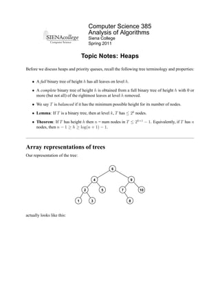
Array representations of trees
Our representation of the tree:
6
4 9
2 5 7 10
1 3 8
actually looks like this:

2. CS 385 Analysis of Algorithms Spring 2011
6
4 9
2 5 E E 7 E 10 E E
1 E E 3 E E 8 E E
= null reference
E = reference to unique EMPTY tree
That’s a lot of extra references to parents and children, and to empty nodes. So to store 10 actual
data values, we need space for 40 references plus the 4 that make up the empty tree instances.
The following array contains exactly the same information:
0 1 2 3 4 5 6 7 8 9 10 11 12 13 14
6 4 9 2 5 7 10 1 3 8
The array, data[0..n-1], holds the values to be stored in the tree. It does not contain explicit
references to the left or right subtrees or to parents.
Instead the children of node i are stored in positions 2 ∗ i + 1 and 2 ∗ i + 2, and therefore the parent
of a node j, may be found at (j − 1)/2
This lets us save space for links, but it is possible that there is a significant waste of storage:
Storing a tree of height n requires an array of length 2(n+1) − 1 (!), even if the tree only has Θ(n)
elements. So this representation is very expensive if you have a long, skinny tree. However, it is
very efficient for holding full or complete trees. For our example, we need 15 references to hold a
tree of 10 items, compared to 40 for the fully constructed binary tree.
Heaps and Priority Queues
First, we’ll consider a structure that seems somewhat like an ordered structure and somewhat like
a queue:
A priority queue is a structure where the contents are comparable elements and the elements with
“small” (or “large”) values are removed before elements with “larger” (or “smaller”) values.
Waiting at a restaurant can be a priority queue – you get in line but people who are regular cus-
tomers or who give a tip to the host or hostess may move ahead of you in line.
2

3. CS 385 Analysis of Algorithms Spring 2011
Same idea when airports are backed up. Planes will get in line for their turn on the runway, but
scheduling concerns or fuel issues or whatever else may cause ground control to give a plane which
“got in line” later a higher priority and move them up.
An operating system may be scheduling processes that are competing to use the CPU in a multi-
programmed system. The next process may be selected based on the highest prioirty process that
is seeking a turn on the CPU.
Much like stacks and traditional queues, we only need to define a single add and remove method.
We can add any element at any time, but we can only ever examine or remove the smallest item.
One can implement a priority queue sort of like a regular queue, but where either you work harder
to insert or to remove an element (i.e., store in priority order – maintain a sorted internal stucture,
or search each time to remove lowest priority elements).
We can implement a priority queue using an array or ArrayList or some sort of linked list, but
in any case, at least one of add or remove will be a linear time operation. (Which one is Θ(n)
depends on which scheme is adopted!)
But... we can do better. Using the observation that we don’t need to keep the entire structure
ordered – at any time we only need quick access to the smallest element – we can provide a more
efficient implementation using a structure called at heap.
Recall that a complete binary tree is one in which every level is full except possibly the bottom
level and that level has all leaves in the leftmost positions. (Note that this is more restrictive than a
balanced tree.)
Definition: A Min-Heap H is a complete binary tree such that
1. H is empty, or
2. (a) The root value is the smallest value in H and
(b) The left and right subtrees of H are also heaps
This is equivalent to saying that H[i] <= H[2*i+1], and H[i] <= H[2*i+2] for all ap-
propriate values of i in the array representation of trees.
We could just as well implement a Max-Heap – just reverse all of our comparisons. The text in
fact does talk about max heaps.
In either case, it often makes sense to use the array/ArrayList representation of binary trees
here, since the tree is also guaranteed to be complete, so there will never be empty slots wasting
space.
Another way of looking at Min-Heap is that any path from a leaf to the root is in non-ascending
order.
3

4. CS 385 Analysis of Algorithms Spring 2011
1
4 2
6 5 10 3
9 7 8
Note that there are lots of possible Min-Heaps that would contain the same set of values. At
each node, the subtrees are interchangeable (other than those which have different heights, strictly
speaking).
In a Min-heap, we know that the smallest value is at the root, the second smallest is a child of the
root, the third smallest is a child of the first or second smallest, and so on.
This turns out to be exactly what is needed to implement a priority queue.
We need to be able to maintain a Min-Heap, and when elements are added or the smallest value is
removed, we want to “re-heapify” the structure as efficiently as possible.
Inserting into a Heap
1. Place number to be inserted at the next free position.
2. “Percolate” it up to correct position.
Deleting the Root from a Heap
1. Save value in root element for return (it’s the smallest one).
2. Move last element to root
3. Push down (or “sift”) the element now in the root position (it was formerly the last
element) to its correct position by repeatedly swapping it with the smaller of its two
children.
Notice how these heap operations implement a priority queue.
When you add a new element in a priority queue, copy it into the next free position of the heap and
sift it up into its proper position.
When you remove the next element from the priority queue, remove the element from the root of
heap (first elt, since it has lowest number for priority), move the last element up to the first slot,
and then sift it down.
If we implement a priority queue using a heap and store our heap in array/ArrayList format,
the add and remove operations can both be implemented efficiently.
4

5. CS 385 Analysis of Algorithms Spring 2011
Removing an element involves getting the smallest, removing it from the start of the array, and
“heapifying” the remaining values. As we did in the example, we remove the first value, move up
the last value to that first position, and “sift” it down to a valid position.
The add operation is pretty straightforward. Just put it at the end of the array and “percolate” it
up to restore the heap condition.
How expensive are these “percolate up” and “push down root” operations?
Each is Θ(log n), as we can, at worst, traverse the height of the tree. Since the tree is always
complete, we know its height is always at most log n. This is much better than storing the priority
queue as regular queue and inserting new elements into the right position in the queue and removing
them from the front.
Sorting with a Heap (HeapSort)
The priority queue suggests an approach to sorting data. If we have n values to sort, we can add
them all to the priority queue, then remove them all, and they come out in order. We’re done.
What is the cost of this? If we use the naive priority queue implementations (completely sorted
or completely unsorted internal data, making either add or remove Θ(n) and the other Θ(1)), we
need, at some point, to do a Θ(n) operation for each of n elements, making an overall sorting
procedure of Θ(n2 ). That’s not very exciting – we had that with a bubble sort.
But what about using the heap-based priority queues?
We can build a heap from a collection of objects by adding them one after the other. Each takes at
most O(log n) to insert and “percolate up” for a total time of O(n log n) to “heapify” a collection
of numbers. That’s actually the cost of the entire sorting procedure for merge sort and quicksort,
and here, we’ve only achieved a heap, not a sorted structure. But we continue..
Once the heap is established, we remove elements one at a time, putting smallest at end, second
smallest next to end, etc. This is again n steps, each of which is at most an O(log n) operation.
So we have an overall cost of O(n log n), just like our other good sorting procedures.
We can actually do a little better on the “heapify” part. Consider this example, which I will draw
as a tree, but we should remember that it will really just all be in an array or an ArrayList.
25
46 19
58 21 23 12
We want to heapify. Note that we already have 4 heaps – the leaves:
5

6. CS 385 Analysis of Algorithms Spring 2011
25
46 19
58 21 23 12
We can make this 2 heaps by “sifting down” the two level 1 nodes:
25
21 12
58 46 23 19
Then finally, we sift down the root to get a single heap:
12
21 19
58 46 23 25
How expensive was this operation, really?
We only needed to do the “push down root” operation on about half of the elements. But that’s still
O(n) operations, each costing O(log n).
The key is that we only perform “push down root” on the first half of the elements of the array.
That is, no “push down root” operations are needed corresponding to leaves of the tree (corre-
sponding to n of the elements).
2
For those elements sitting just above the leaves ( n of the elements), we only go through the loop
4
once (and thus we make only two comparisons of priorities).
For those in the next layer ( n of the elements) we only go through the loop twice (4 comparisons),
8
and so on.
Thus we make
n n n
2 ∗ ( ) + 4 ∗ ( ) + 6 ∗ ( ) + · · · + 2 ∗ (log n) ∗ (1)
4 8 16
total comparisons.
Since 2log n = n, we can rewrite the last term to fit in nicely:
6

7. CS 385 Analysis of Algorithms Spring 2011
n n n n
2 ∗ ( ) + 4 ∗ ( ) + 6 ∗ ( ) + · · · + 2 ∗ (log n) ∗ ( log n )
4 8 16 2
We can factor out the n, multiply in the 2 (to reduce each denominator by 2) and put things into a
more suggestive format:
1 2 3 log n
n∗ 1
+ 2 + 3 + · · · + log n
2 2 2 2
The sum inside the parentheses can be rewritten as
log n
i
i=1 2i
This is clearly bounded above by the infinite sum,
∞
i
i
i=1 2
Let’s see if we can evaluate this infinite sum:
1 2 3 4
+ + + +···
2 4 8 16
We can rewrite this in a triangular form to be able to use some tricks to get the sum:
1 1 1 1
+ + + +··· = 1
2 4 8 16
1 1 1 1
+ + +··· =
4 8 16 2
1 1 1
+ +··· =
8 16 4
1 1
+··· =
16 8
1
··· =
16
···
2
Thus
1 2 3 log n
n∗( + 2 + 3 + · · · + log n ) <= 2n
21 2 2 2
and hence the time to heapify an array or ArrayList, in place, is Θ(n).
7

8. CS 385 Analysis of Algorithms Spring 2011
The second phase, removing each successive element, still requires n removes, each of which will
involve a Θ(log n) heapify.
We can, however, do this in place in our array or ArrayList, by swapping each element removed
from the heap into the last position in the heap and calling the heap one item smaller at each step.
25
21 19
58 46 23 12
And then we do a sift down of the root (which just came up from the last position):
19
21 23
58 46 25 12
Then the next item (19) comes out of the heap by swapping into the last position, and we sift down
the 25:
21
25 23
58 46 19 12
And the process continues until there is no more heap.
The entire process of extracting elements in sorted order is Θ(n log n).
Therefore, the total time is Θ(n log n).
Plus, there’s no extra space needed!
Note that using a Min-Heap, we end up with the array sorted in descending order. If we want to
sort in ascending order, we will need a Max-Heap.
So we have a new efficient sorting procedure to add to our arsenal.
8