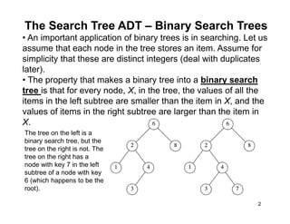
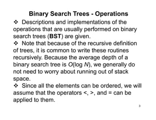
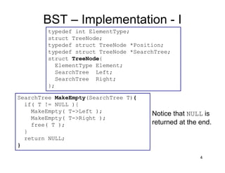
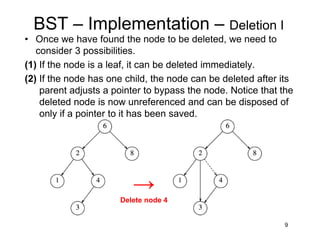
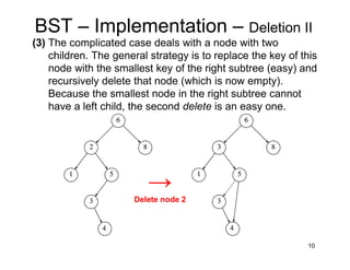
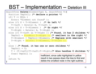
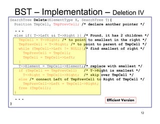
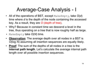
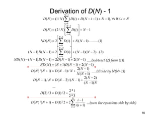
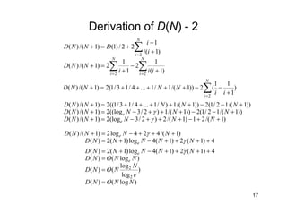
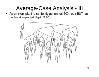
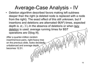
This document discusses binary search trees (BSTs). It describes how BSTs are structured, with each node containing a value greater than all values in its left subtree and less than all values in its right subtree. It then summarizes common BST operations like insertion, deletion, finding minimum/maximum values, and provides pseudocode implementations. The average-case runtime of these operations is analyzed, showing that since the average depth of a BST is O(log N), most operations take O(log N) time on average. Repeated insertions and deletions can cause imbalance and increase the average depth to O(√N).

1. Chapter 4: Trees (BST)
Text: Read Weiss, §4.3
1

2. The Search Tree ADT – Binary Search Trees
2
• An important application of binary trees is in searching. Let us
assume that each node in the tree stores an item. Assume for
simplicity that these are distinct integers (deal with duplicates
later).
• The property that makes a binary tree into a binary search
tree is that for every node, X, in the tree, the values of all the
items in the left subtree are smaller than the item in X, and the
values of items in the right subtree are larger than the item in
X.
The tree on the left is a
binary search tree, but the
tree on the right is not. The
tree on the right has a
node with key 7 in the left
subtree of a node with key
6 (which happens to be the
root).

3. 3
Binary Search Trees - Operations
Descriptions and implementations of the
operations that are usually performed on binary
search trees (BST) are given.
Note that because of the recursive definition
of trees, it is common to write these routines
recursively. Because the average depth of a
binary search tree is O(log N), we generally do
not need to worry about running out of stack
space.
Since all the elements can be ordered, we will
assume that the operators <, >, and = can be
applied to them.

4. BST – Implementation - I
4
typedef int ElementType;
struct TreeNode;
typedef struct TreeNode *Position;
typedef struct TreeNode *SearchTree;
struct TreeNode{
ElementType Element;
SearchTree Left;
SearchTree Right;
};
SearchTree MakeEmpty(SearchTree T){
if( T != NULL ){
MakeEmpty( T->Left );
MakeEmpty( T->Right );
free( T );
}
return NULL;
}
Notice that NULL is
returned at the end.

5. 5
• Find operation generally requires returning a pointer to the node in
the Binary Search Tree pointed by T that has value X, or NULL if there
is no such node. The structure of the tree makes this simple. If T is
NULL , then we can just return . Otherwise, we make a recursive call
on either the left or the right subtree of the node pointed by T,
depending on the relationship of X to the value stored in the node
pointed by T. Otherwise, if the value stored X, we can return T.
Position Find(ElementType X, SearchTree T){
if( T == NULL )
return NULL;
if( X < T->Element )
return Find( X, T->Left );
else if( X > T->Element )
return Find( X, T->Right );
else
return T;
}
BST – Implementation - II

6. 6
Position FindMin(SearchTree T){
if( T == NULL )
return NULL;
else if( T->Left == NULL )
return T;
else
return FindMin( T->Left );
}
Position FindMax(SearchTree T){
if( T != NULL )
while( T->Right != NULL )
T = T->Right;
return T;
}
BST – Implementation - III
•To perform a FindMin, start at
the root and go left as long as
there is a left child. The stopping
point is the smallest element.
•The FindMax routine is the
same, except that branching is to
the right child.
•Notice that the degenerate case
of an empty tree is carefully
handled.
•Also notice that it is safe to
change T in FindMax, since we
are only working with a copy.
Always be extremely careful,
however, because a statement
such as
T->right=T->right->right
will make changes.

7. 7
BST – Implementation – Insertion I
The insertion routine is conceptually simple. To insert X into tree T,
proceed down the tree as you would with a Find. If X is found, do
nothing (or "update" something). Otherwise, insert X at the last spot
on the path traversed. Duplicates can be handled by keeping an extra
field in the node indicating the frequency of occurrence. If the key is
only part of a larger record, then all of the records with the same key
might be kept in an auxiliary data structure, such as a list or another
search tree.
→
Insert node 5

8. 8
SearchTree Insert(ElementType X, SearchTree T){
if( T == NULL ){
/* Create and return a one-node tree */
T = malloc( sizeof( struct TreeNode ) );
if( T == NULL )
FatalError( "Out of space!!!" );
else {
T->Element = X;
T->Left = T->Right = NULL;
}
}
else if( X < T->Element )
T->Left = Insert( X, T->Left );
else if( X > T->Element )
T->Right = Insert( X, T->Right );
/* Else X is in the tree already; do nothing */
return T; /* Do not forget this line!! */
}
BST – Implementation – Insertion II

9. 9
BST – Implementation – Deletion I
• Once we have found the node to be deleted, we need to
consider 3 possibilities.
(1) If the node is a leaf, it can be deleted immediately.
(2) If the node has one child, the node can be deleted after its
parent adjusts a pointer to bypass the node. Notice that the
deleted node is now unreferenced and can be disposed of
only if a pointer to it has been saved.
→
Delete node 4

10. 10
BST – Implementation – Deletion II
(3) The complicated case deals with a node with two
children. The general strategy is to replace the key of this
node with the smallest key of the right subtree (easy) and
recursively delete that node (which is now empty).
Because the smallest node in the right subtree cannot
have a left child, the second delete is an easy one.
→
Delete node 2

11. 11
BST – Implementation – Deletion III
SearchTree Delete(ElementType X, SearchTree T){
Position TmpCell; /* declare a pointer */
if( T == NULL )
Error( "Element not found" );
else if( X < T->Element ) /* Go left */
T->Left = Delete( X, T->Left );
else if( X > T->Element ) /* Go right */
T->Right = Delete( X, T->Right );
else if( T->Left && T->Right ){ /* Found, it has 2 children */
TmpCell = FindMin( T->Right ); /* smallest in the right */
T->Element = TmpCell->Element; /* Replace with smallest */
T->Right = Delete( T->Element, T->Right );
}
else { /* Found, it has one or zero children */
TmpCell = T;
T = (T->Left)?T->Left:T->Right;/* Also handles 0 children */
free( TmpCell );
}
return T;
}
Inefficient, since calls highlighted in yellow
result in two passes down the tree to find and
delete the smallest node in the right subtree.

12. • We can use stacks to convert an
expression in standart form (otherwise
known as infix) into postfix.
• Example: operators = {+, *, (, )}, usual
precedence rules; a + b * c + (d * e + f) * g
Answer = a b c * + d e * f + g * +
12
BST – Implementation – Deletion IV
SearchTree Delete(ElementType X, SearchTree T){
Position TmpCell, TmpPrevCell; /* declare another pointer */
...
else if( T->Left && T->Right ){ /* Found, it has 2 children */
TmpCell = T->Right; /* to point to smallest in the right */
TmpPrevCell = T->Right; /* to point to parent of TmpCell */
while (TmpCell->Left != NULL){/* find smallest of right */
TmpPrevCell = TmpCell;
TmpCell = TmpCell->Left;
}
T->Element = TmpCell->Element;/* replace with smallest */
if (TmpCell == TmpPrevCell) /* T->Right is smallest */
T->Right = TmpCell->Right; /* skip over TmpCell */
else /* connect Left of TmpPrevCell to Right of TmpCell */
TmpPrevCell->Left = TmpCell->Right;
free (TmpCell);
}
...
}
Efficient Version

13. BST – Implementation – Lazy Deletion
• If the number of deletions is small, then a popular
strategy to use is lazy deletion: When an element is
to be deleted, it is left in the tree and merely marked
as deleted. This is especially popular if duplicates are
present, because then the field that keeps count of
the items can be decremented.
• If the number of real nodes is the same as the
number of "deleted" nodes, then the depth of the tree
is only expected to go up by a small constant (why?),
so there is a very small time penalty associated with
lazy deletion. Also, if an item is reinserted, the
overhead of allocating a new cell is avoided.
13

14. Average-Case Analysis - I
14
• All of the operations of BST, except MakeEmpty, take O(d)
time where d is the depth of the node containing the accessed
key. As a result, they are O (depth of tree).
• Why? Because in constant time we descend a level in the
tree, thus operating on a tree that is now roughly half as large.
• MakeEmpty take O(N) time.
• Observation: The average depth over all nodes in a BST is
O(log N) assuming all insertion sequences are equally likely.
• Proof: The sum of the depths of all nodes in a tree is the
internal path length. Let’s calculate the average internal path
length over all possible insertion sequences.

15. 15
Average-Case Analysis - II
• Let D(N) be the internal path length for some BST T of N
nodes. D(1) = 0.
• D(N) = D(i) + D(N-i-1) + N -1 // Subtree nodes are 1 level deeper
• All subtree sizes are equally likely for BSTs, since it depends
only on the rank of the first element inserted into BST. This
does not hold for binary trees though. Let’s, then, average:
1)()/2()(
0),1)1()(()/1()(
1
0
1
0
−+



=
<≤∀−+−−+=
∑
∑
−
=
−
=
NiDNND
NiiNiNDiDNND
N
i
N
i
• If the recurrence is solved, D(N) = O(N log N). Thus, the
expected depth of any node is O(log N).

16. Derivation of D(N) - 1
16
1)()/2()(
0),1)1()(()/1()(
1
0
1
0
−+





=
<≤∀−+−−+=
∑
∑
−
=
−
=
NiDNND
NiiNiNDiDNND
N
i
N
i
)1(2)1(2)1()1()(
)2)...(2)(1()(2)1()1(
)1..().........1()(2)(
2
0
1
0
−+−=−−−
−−+





=−−
−+





=
∑
∑
−
=
−
=
NNDNDNNND
NNiDNDN
NNiDNND
N
i
N
i
∑=
+
−
+=+
+=
−
−
+−−=−
+
−
+−=+
−+−+=
N
i
ii
i
DNND
DD
NN
N
NNDNND
NN
N
NNDNND
NNDNNND
2
)1(
1
22/)1()1/()(
3*2
1*2
2/)1(3/)2(
...
)1(
)2(2
)1/()2(/)1(
)1(
)1(2
/)1()1/()(
)1(2)1()1()(
...(sum the equations side by side)
.....(divide by N(N+1))
.....(subtract (2) from (1))

17. 17
Derivation of D(N) - 2
∑∑
∑
==
=
+
−
+
=+
+
−
+=+
N
i
N
i
N
i
iii
NND
ii
i
DNND
22
2
)1(
1
2
1
1
2)1/()(
)1(
1
22/)1()1/()(
∑=
+
−−+++++=+
N
i
ii
NNNND
2
)
1
11
(2))1/(1/1...4/13/1(2)1/()(
)1/(21)1/(2)2/3(log2)1/()(
))1/(12/1(2))1/(1)2/3((log2)1/()(
))1/(12/1(2))1/(1)/1...4/13/1((2)1/()(
++−+++−=+
+−−+++−=+
+−−+++++=+
NNNNND
NNNNND
NNNNND
e
e
γ
γ
4)1(2)1(4log)1(2)(
)1/(424log2)1/()(
++++−+=
+++−=+
NNNNND
NNNND
e
e
γ
γ
)log()(
)
log
log
()(
)log()(
4)1(2)1(4log)1(2)(
2
2
NNOND
e
N
NOND
NNOND
NNNNND
e
e
=
=
=
++++−+= γ

18. 18
Average-Case Analysis - III
• As an example, the randomly generated 500 node BST has
nodes at expected depth 9.98.

19. 19
Average-Case Analysis - IV
)( Nθ
After a quarter-million random
insert/remove pairs, right-heavy tree
on the previous slide, looks decidedly
unbalanced and average depth
becomes 12.51.
• Deletion algorithm described favors making left subtrees
deeper than the right (a deleted node is replaced with a node
from the right). The exact effect of this still unknown, but if
insertions and deletions are alternated Ɵ(N2) times, expected
depth is .In the absence of deletions or when lazy
deletion is used; average running times for BST
operations are O(log N).