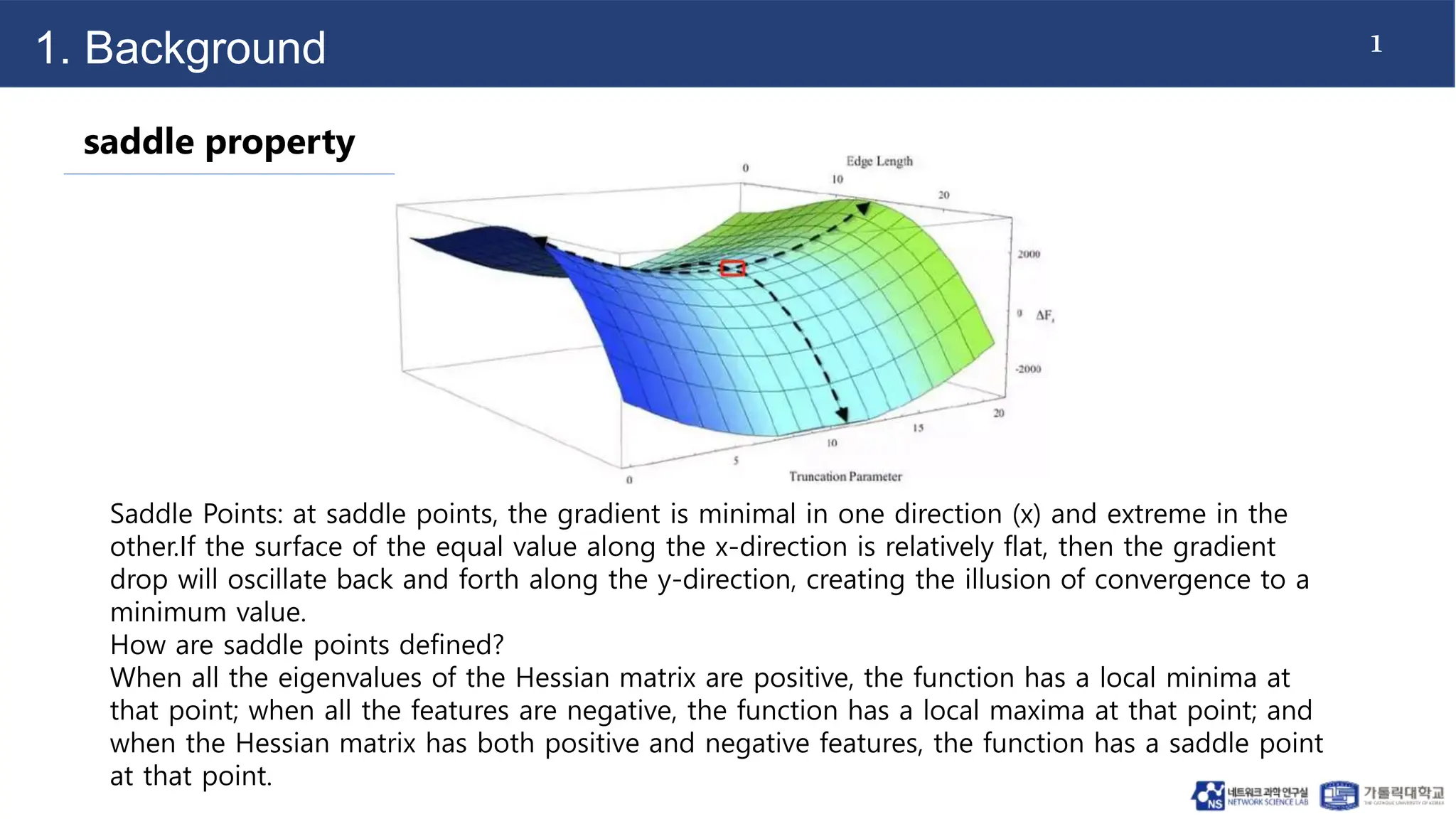
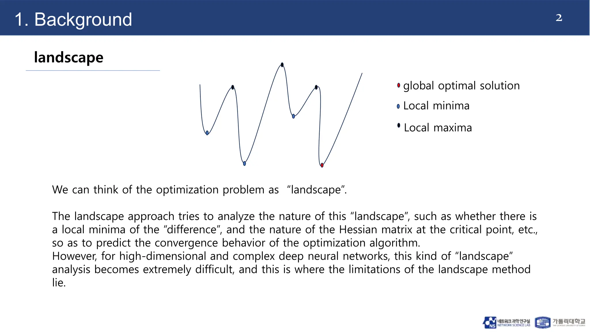
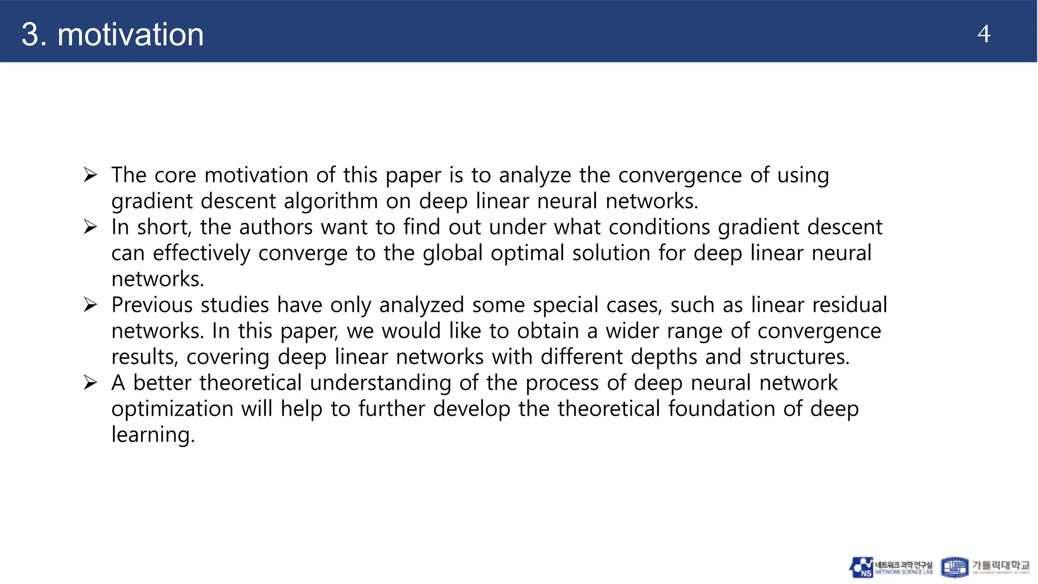
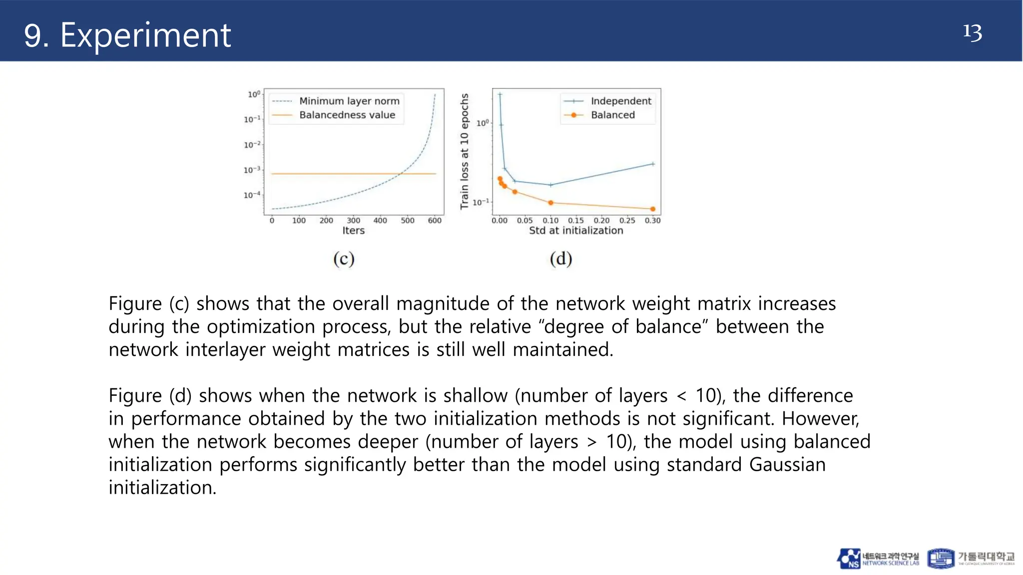
The document discusses the analysis of convergence in gradient descent algorithms applied to deep linear neural networks, emphasizing the importance of weight initialization and conditions that ensure effective convergence to global optimal solutions. It addresses limitations in conventional landscape approaches for deep networks and introduces concepts like approximate balancedness and deficiency margin to facilitate better understanding and optimization. The findings suggest that maintaining balanced weight matrices during initialization enhances convergence speed, especially in deeper networks.

1. YANJUN WU
Network Science Lab
Dept. of Artificial Intelligence
The Catholic University of Korea
E-mail:wuyanjun@catholic.ac.kr

2. 1
Saddle Points: at saddle points, the gradient is minimal in one direction (x) and extreme in the
other.If the surface of the equal value along the x-direction is relatively flat, then the gradient
drop will oscillate back and forth along the y-direction, creating the illusion of convergence to a
minimum value.
How are saddle points defined?
When all the eigenvalues of the Hessian matrix are positive, the function has a local minima at
that point; when all the features are negative, the function has a local maxima at that point; and
when the Hessian matrix has both positive and negative features, the function has a saddle point
at that point.
1. Background
saddle property

3. 2
1. Background
We can think of the optimization problem as “landscape”.
The landscape approach tries to analyze the nature of this “landscape”, such as whether there is
a local minima of the “difference”, and the nature of the Hessian matrix at the critical point, etc.,
so as to predict the convergence behavior of the optimization algorithm.
However, for high-dimensional and complex deep neural networks, this kind of “landscape”
analysis becomes extremely difficult, and this is where the limitations of the landscape method
lie.
global optimal solution
Local minima
Local maxima
landscape

4. 3
2. Introduction
Deep learning is built on top of gradient optimization
methods. Currently the mainstream landscape approach,
which focuses on the special properties of key points
(i.e., points where the gradient of the objective function
is zero), which guarantee convergence to the globally
optimal solution. However, for deep networks, these
special properties are unlikely to hold, so the landscape
approach has limitations in proving the convergence to
the global optimal solution for deep networks.

5. 4
3. motivation
 The core motivation of this paper is to analyze the convergence of using
gradient descent algorithm on deep linear neural networks.
 In short, the authors want to find out under what conditions gradient descent
can effectively converge to the global optimal solution for deep linear neural
networks.
 Previous studies have only analyzed some special cases, such as linear residual
networks. In this paper, we would like to obtain a wider range of convergence
results, covering deep linear networks with different depths and structures.
 A better theoretical understanding of the process of deep neural network
optimization will help to further develop the theoretical foundation of deep
learning.

6. 5
5. Gradient descent
This is the loss function, and the smaller the value of the loss function, the more accurate the mo
del will be. If we want to improve the accuracy of the machine learning model, we need to reduce
the value of the loss function as much as possible. And to reduce the value of the loss function, w
e generally use gradient desce
nt as a method. So, the purpose of gradient descent is to minimize the loss function.
In linear regression we can write:
“F” for Frobenius Paradigm. ||A||F = sqrt(sum of squares of all elements of matrix A)

7. 6
5. Gradient descent
is the empirical (uncentered) cross-covariance matrix between instances and labels, an
d 𝑐 is a constant (that does not depend on 𝑊). Denoting

8. 7
5. Gradient descent
This formula can also be written as:
where the formula for updating the gradient can be expressed as:
This formula represents the definition of the loss function ℓ:
In this formulation, the loss function ℓ is decomposed into n components ℓ₁(θ), ℓ₂(θ), ... , ℓₙ(θ).
Each component represents the part of the loss function with respect to the corresponding
parameter. This decomposition can help us analyze and optimize the loss function.

9. 8
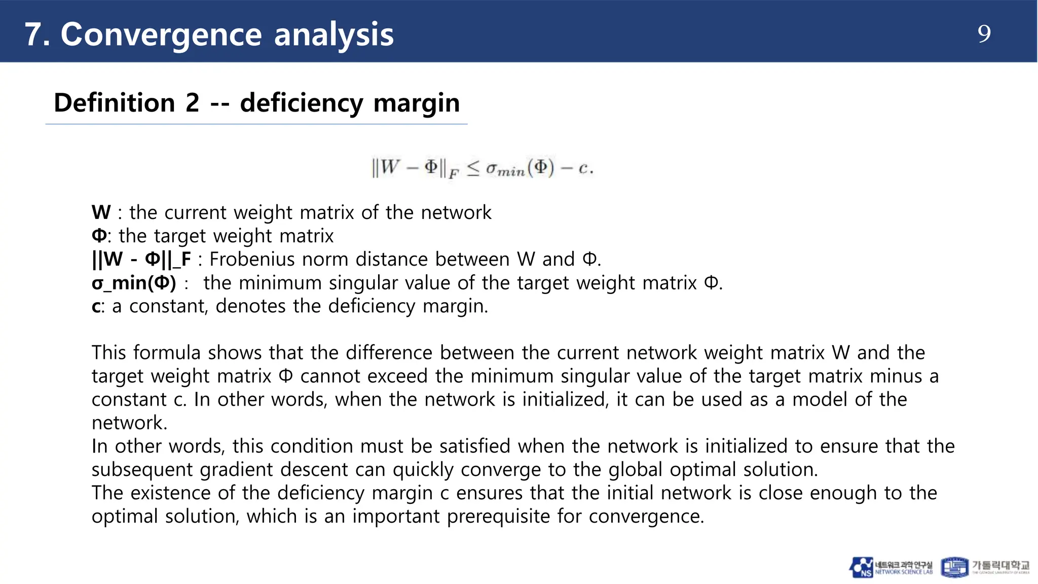
7. Convergence analysis
Definition 1 -- approximate balancedness
approximate balancedness means that the ratio of the singular values of the weight matrix
for each layer cannot be too large.
W1 shape: torch.Size([3, 5])
W2 shape: torch.Size([2, 3])
||[3,2]·[2,3]-[3,5]·[5,3]||F≤ δ
The smaller δ is, the more uniform the distribution of singular values of this weight matrix is,
and the closer to the " balance " state.
W1 W2

10. 9
Definition 2 -- deficiency margin
W : the current weight matrix of the network
Φ: the target weight matrix
||W - Φ||_F : Frobenius norm distance between W and Φ.
σ_min(Φ)： the minimum singular value of the target weight matrix Φ.
c: a constant, denotes the deficiency margin.
This formula shows that the difference between the current network weight matrix W and the
target weight matrix Φ cannot exceed the minimum singular value of the target matrix minus a
constant c. In other words, when the network is initialized, it can be used as a model of the
network.
In other words, this condition must be satisfied when the network is initialized to ensure that the
subsequent gradient descent can quickly converge to the global optimal solution.
The existence of the deficiency margin c ensures that the initial network is close enough to the
optimal solution, which is an important prerequisite for convergence.
7. Convergence analysis

11. 10
8. Main theorem-1
These two formulas are derived based on Theorem 1 and Theorem 2
1. The step size needs to satisfy an upper bound that grows larger as the network gets
deeper, and is related to the number of norms in the initial weight matrix.
2. There is also a lower bound on the number of iterations needed for gradient descent,
which increases as the network gets deeper, and is also related to the step size and the
initial loss value.

12. 11
8. Main theorem-2
 Step size η: The smaller the step size, the larger the minimum number of iterations T
required. This reflects the tradeoff between step size and convergence speed.
 Initial loss d0: The larger the initial loss d0, the larger the number of iterations T. In other
words, the smaller the initial loss, the larger the number of iterations T. The smaller the
initial loss, the greater the convergence speed. In other words, the smaller the initial loss
value, the faster the convergence.
 Weight Matrix Paradigm “Φ”: The larger the weight matrix paradigm, the larger the
number of iterations T. This again emphasizes the importance of weight initialization. This
again highlights the importance of weight initialization.
 Network Depth N: As the network depth N increases, the number of iterations T
increases. This indicates that for deeper networks, more iterations are required for
convergence.

13. 12
9. Experiment
X:Weight initialization using Gaussian distribution
Y:number of iterations required to train the loss down to a threshold of 10^-5
(a) Using the normal Gaussian distribution.
(b) Using the “approximate balancedness” method proposed in the paper in addition
to (a).
In contrast to the standard Gaussian initialization (Fig. 1a) which can only converge
fast over a narrow range of initialization standard deviations. Using the approximate
balancedness proposed in the paper (Fig. 1b) can maintain faster training convergence
over a wider range of initialization standard deviations.

14. 13
9. Experiment
Figure (c) shows that the overall magnitude of the network weight matrix increases
during the optimization process, but the relative “degree of balance” between the
network interlayer weight matrices is still well maintained.
Figure (d) shows when the network is shallow (number of layers < 10), the difference
in performance obtained by the two initialization methods is not significant. However,
when the network becomes deeper (number of layers > 10), the model using balanced
initialization performs significantly better than the model using standard Gaussian
initialization.

15. 14
10. Conclusion
The dimension of the hidden layer should be at least equal to the
minimum of the input and output dimensions. This is to ensure that the
network has enough expressive power to avoid information bottlenecks.
At initialization, the weight matrix of the network should be
approximately balanced. That is to say, the weight magnitude of each
layer should be relatively balanced, and there should be no obvious
asymmetry.
After using the appropriate balanced initialization method, the initial loss
function value should be smaller than the loss of any rank-loss solution.
This means that the initial state of the network is already better than the
severely underfitted model.

16. 15
4. Question
Q&A