Downloaded 950 times


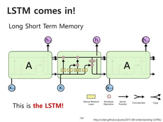
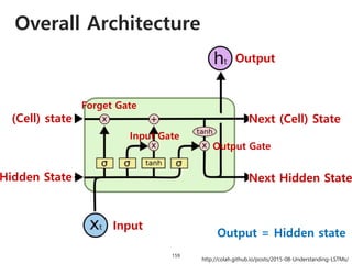
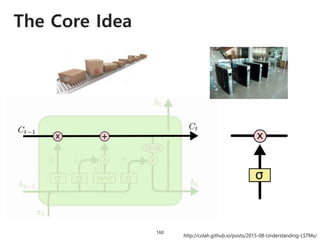

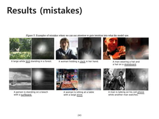
![Solving VQA
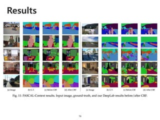
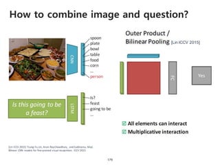
163
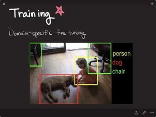
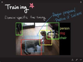
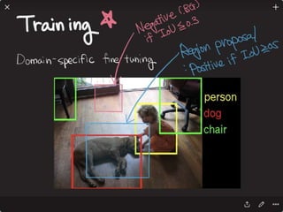
Approach
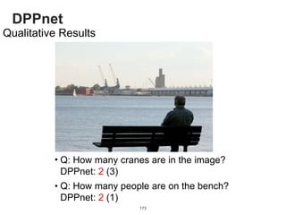
[Malinowski et al., 2015] [Ren et al., 2015] [Andres et al., 2015]
[Ma et al., 2015] [Jiang et al., 2015]
Various methods have been proposed](https://image.slidesharecdn.com/dlincv-161110052148/85/Deep-Learning-in-Computer-Vision-163-320.jpg)
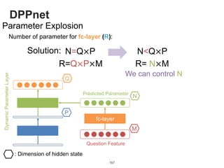
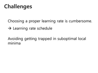
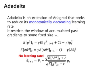
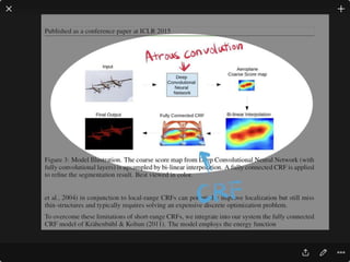
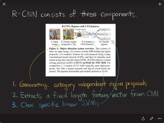
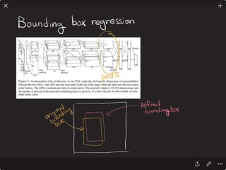
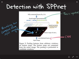
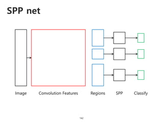
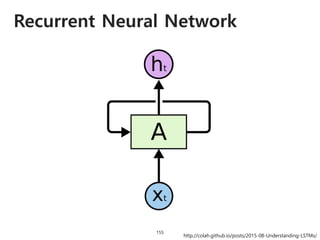
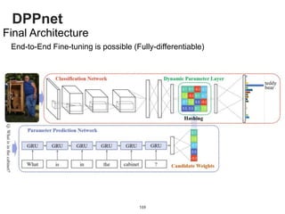
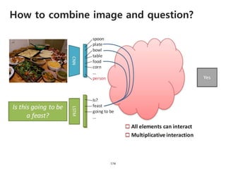
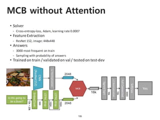
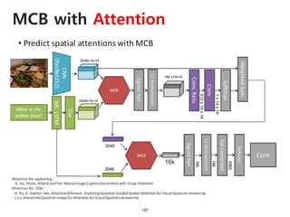
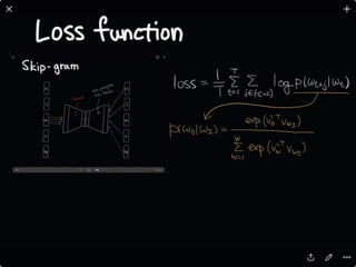
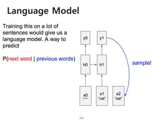
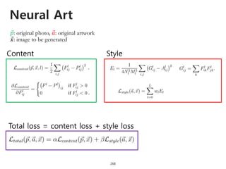
![DPPnet
168
Weight Sharing with Hashing Trick
Weights of Dynamic Parameter Layer are picked from Candidate weights by Hashing
Question Feature
Candidate Weights
fc-layer
0.11.2-0.70.3-0.2
0.1 0.1 -0.2 -0.7
1.2 -0.2 0.1 -0.7
-0.7 1.2 0.3 -0.2
0.3 0.3 0.1 1.2
DynamicParameterLayer
Hasing
[Chen et al., 2015]](https://image.slidesharecdn.com/dlincv-161110052148/85/Deep-Learning-in-Computer-Vision-168-320.jpg)


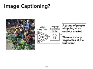
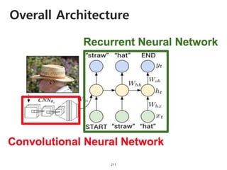


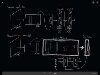
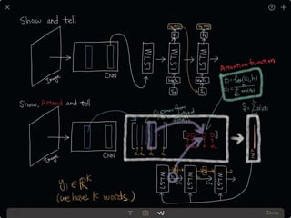


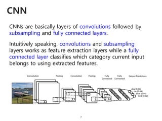
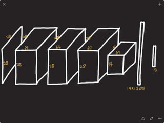
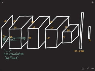
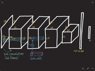
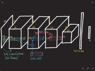
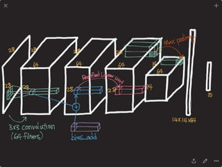
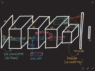
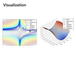
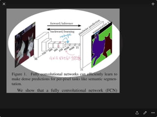
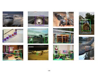
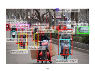
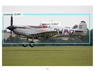
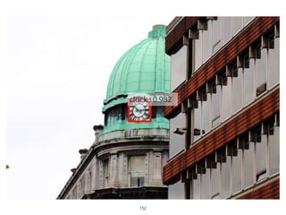
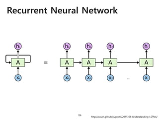
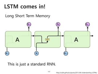
The document provides an introduction to deep learning, covering its fundamental concepts, including optimization methods, the basics of convolutional neural networks (CNNs), recurrent neural networks (RNNs), and their applications in semantic segmentation, weakly supervised localization, and image detection. It discusses various gradient descent algorithms and introduces advanced techniques such as the dynamic parameter prediction network for visual question answering and methods for image captioning. The presentation also highlights the importance of feature extraction and visualization in deep learning processes.