Download as PDF, PPTX
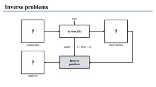

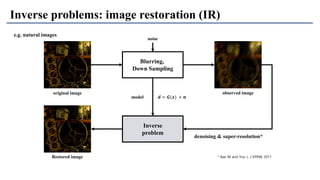
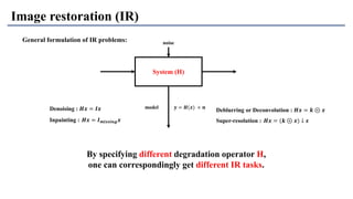
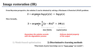
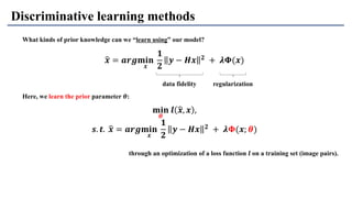
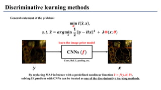
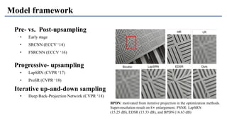
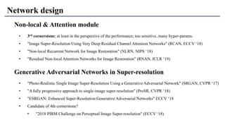
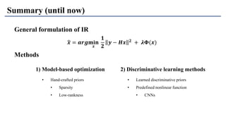
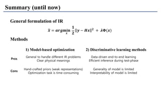
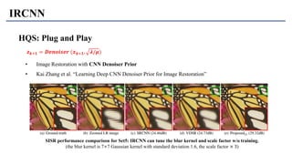
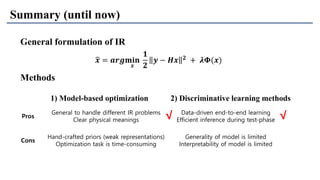
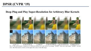

1) The document discusses super-resolution techniques in deep learning, including inverse problems, image restoration problems, and different deep learning models. 2) Early models like SRCNN used convolutional networks for super-resolution but were shallow, while later models incorporated residual learning (VDSR), recursive learning (DRCN), and became very deep and dense (SRResNet). 3) Key developments included EDSR which provided a strong backbone model and GAN-based approaches like SRGAN which aimed to generate more realistic textures but require new evaluation metrics.


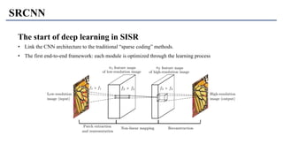
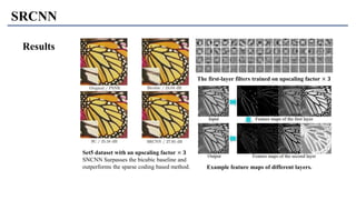
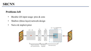
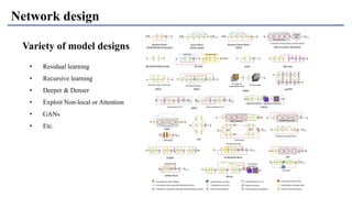
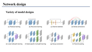
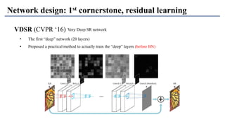
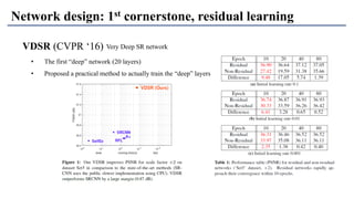
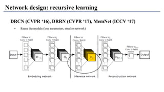
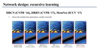
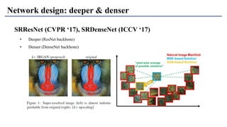
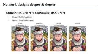
![[OSGeo-KR Tech Workshop] Deep Learning for Single Image Super-Resolution](https://cdn.slidesharecdn.com/ss_thumbnails/osgeo-krdeeplearningforsingleimagesuper-resolution-180223175347-thumbnail.jpg?width=640&height=640&fit=bounds)


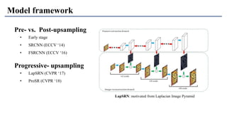
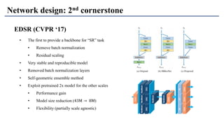
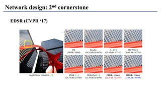
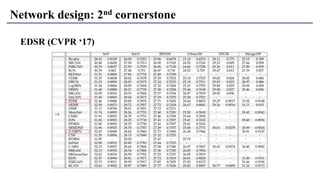
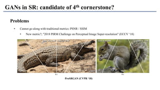
![[PR12] categorical reparameterization with gumbel softmax](https://cdn.slidesharecdn.com/ss_thumbnails/pr12categoricalreparameterizationwithgumbel-softmax-180304131005-thumbnail.jpg?width=640&height=640&fit=bounds)

![[PR12] Inception and Xception - Jaejun Yoo](https://cdn.slidesharecdn.com/ss_thumbnails/pr12inceptionandxception-jaejunyoo-170910140157-thumbnail.jpg?width=640&height=640&fit=bounds)

![[PR12] Capsule Networks - Jaejun Yoo](https://cdn.slidesharecdn.com/ss_thumbnails/pr12capsulenetworks-jaejunyoo-171217144319-thumbnail.jpg?width=640&height=640&fit=bounds)
![[Pr12] dann jaejun yoo](https://cdn.slidesharecdn.com/ss_thumbnails/pr12dann-jaejunyoo-170604150015-thumbnail.jpg?width=640&height=640&fit=bounds)

![[PR12] understanding deep learning requires rethinking generalization](https://cdn.slidesharecdn.com/ss_thumbnails/pr12understandingdeeplearningrequiresrethinkinggeneralization-180121135850-thumbnail.jpg?width=640&height=640&fit=bounds)

![[PR12] Spectral Normalization for Generative Adversarial Networks](https://cdn.slidesharecdn.com/ss_thumbnails/pr12spectralnormalizationforgans-180513142600-thumbnail.jpg?width=640&height=640&fit=bounds)
![[CVPR2020] Simple but effective image enhancement techniques](https://cdn.slidesharecdn.com/ss_thumbnails/simplebuteffectiveimageenhancementtechniques-200617034047-thumbnail.jpg?width=640&height=640&fit=bounds)
![[PR12] Generative Models as Distributions of Functions](https://cdn.slidesharecdn.com/ss_thumbnails/pr12generativemodelsasdistributionsoffunctions-jaejunyoo-210411152822-thumbnail.jpg?width=640&height=640&fit=bounds)
![[PR12] intro. to gans jaejun yoo](https://cdn.slidesharecdn.com/ss_thumbnails/pr12intro-170416162251-thumbnail.jpg?width=640&height=640&fit=bounds)


