Downloaded 2,380 times
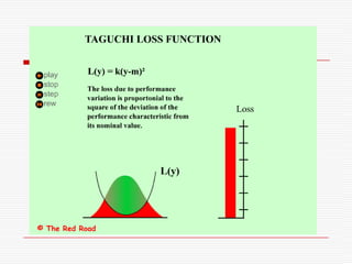
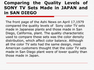
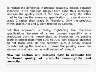
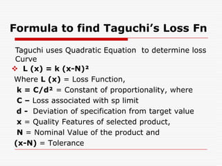
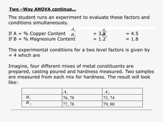
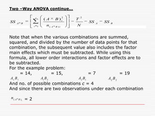
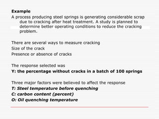
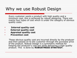
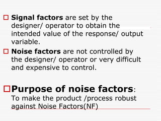
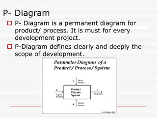
![Taguchi’s method: Loss function..Loss = L(y) = L( m + (y-m)) = L(m) + (y-m) L’(m)/ 1! + (y – m)2 L”(m)/ 2! + …Ideally:(a) L(m) = 0 [if actual size = target size, Loss = 0], and(b) When y = m, the loss is at its minimum, therefore L'(m) = 0Taguchi’s Approximation: L(y) ≈ k( y – m)2](https://image.slidesharecdn.com/taguchimethods-091110232204-phpapp02/85/Seminar-on-Basics-of-Taguchi-Methods-21-320.jpg?cb=1257895364)
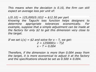
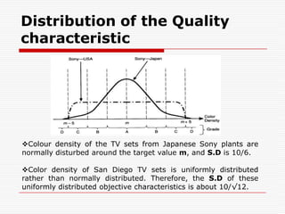
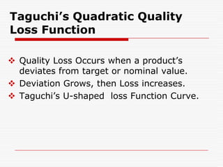
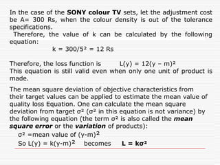
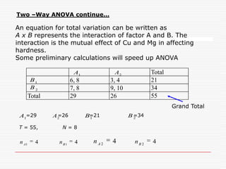
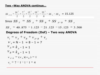
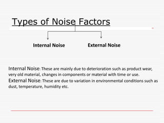
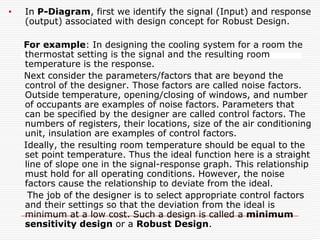
![it is clear that although the defective ratio of the Japanese Sony is higher than that of the San Diego Sony, the quality level of the former is 3 times higher than the latter.If Tighten the toleranceAssume that one can tighten the tolerance specifications of the TV sets of San Diego Sony to be m ± 10/3. Also assume that these TV sets remain uniformly distributed after the tolerance specifications are tightened. The average quality level of San Diego Sony TV sets would be improved to the following quality level: L = 12[(1/ √12) (10) (2/3)] ² = 45Rs](https://image.slidesharecdn.com/taguchimethods-091110232204-phpapp02/85/Seminar-on-Basics-of-Taguchi-Methods-25-320.jpg?cb=1257895364)
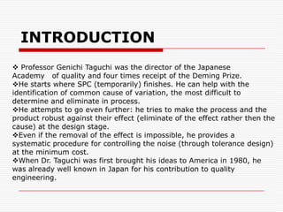
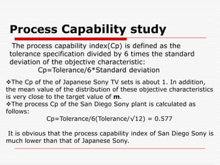
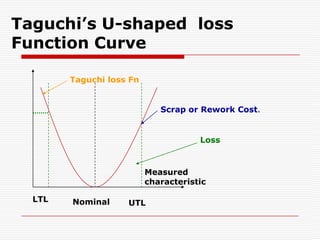
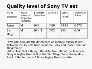
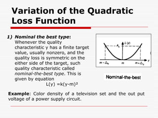
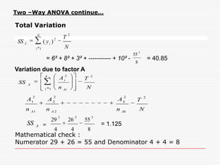
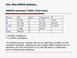
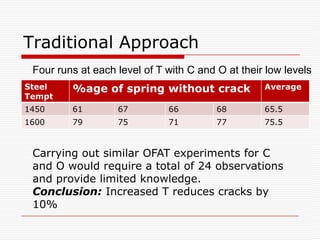
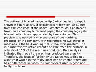
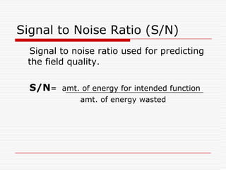
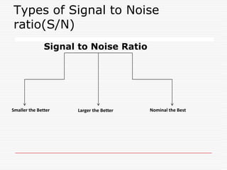
![3)Larger-the-better type: Some characteristics do not take negative values. But, zero is there worst value, and as their value becomes larger, the performance becomes progressively better-that is, the quality loss becomes progressively smaller. ,, also Their ideal value is infinity and at that point the loss is zero. Such characteristics are called larger-the-better type characteristics.Example: Such as the bond strength of adhesives.Thus we approximate the loss function for a larger-the-better type characteristic by substituting 1/y for y in L(y) = k [1/y²]](https://image.slidesharecdn.com/taguchimethods-091110232204-phpapp02/85/Seminar-on-Basics-of-Taguchi-Methods-31-320.jpg?cb=1257895364)
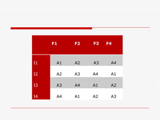
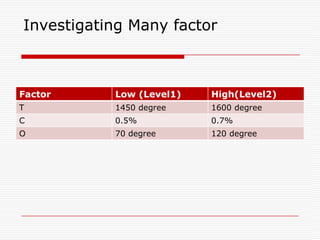

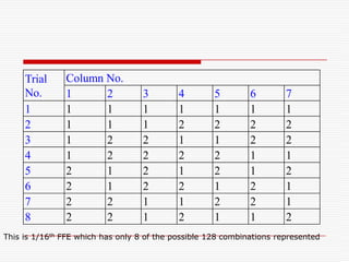

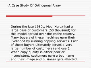
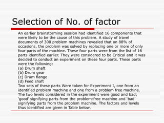
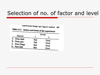
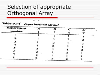
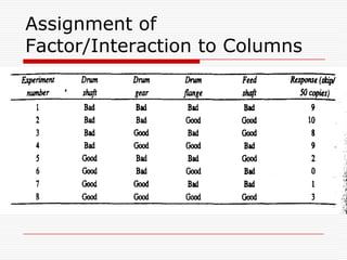
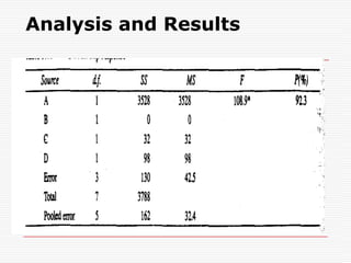

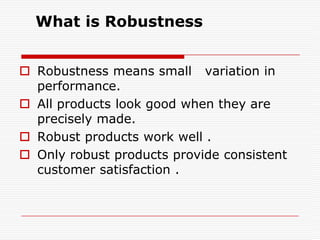
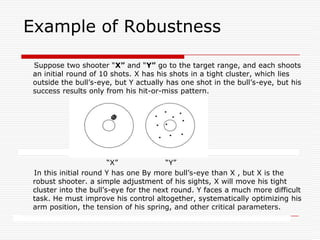
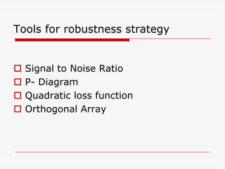


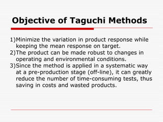
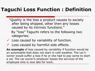
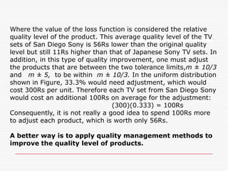
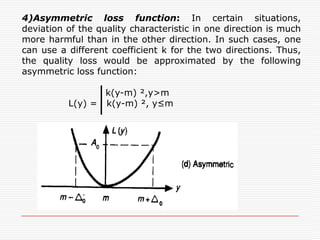
Professor Genichi Taguchi's methods focus on minimizing variation and making processes robust during design stages, emphasizing a quality definition based on societal losses due to product performance deviation. A comparison of Sony TV sets' quality showed that Japanese models had better process capability than those manufactured in San Diego, illustrating the significance of robust quality management. The document also discusses broader statistical methods like ANOVA and the use of orthogonal arrays for optimizing product performance, showing the importance of systematic testing in quality engineering.


![Acceptance Sampling[1]](https://cdn.slidesharecdn.com/ss_thumbnails/acceptancesampling1-1226078569232381-9-thumbnail.jpg?width=640&height=640&fit=bounds)


![Consumer and Producers Risk[1]](https://cdn.slidesharecdn.com/ss_thumbnails/consumerandproducersrisk1-1226081269406229-9-thumbnail.jpg?width=640&height=640&fit=bounds)