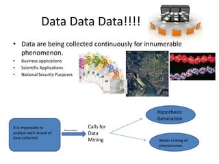
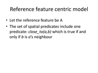
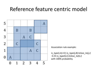
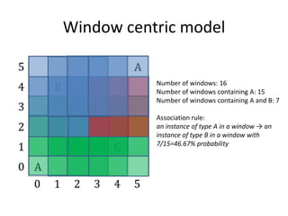
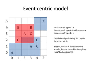
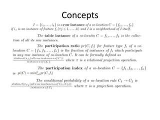
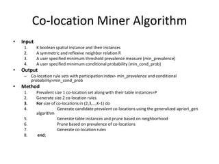
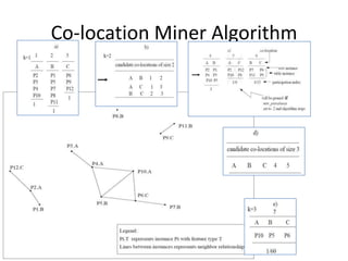
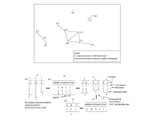
This document summarizes research on discovering spatial co-location patterns from geospatial data. It discusses how spatial data mining differs from classical data mining by considering attribute relationships between neighboring spatial objects. The paper focuses on extracting frequent co-occurrence rules between boolean spatial features from ecological datasets. It presents three approaches for modeling co-location rules problems - reference feature centric, window centric, and event centric. The Co-location Miner algorithm is introduced for mining co-location rules that satisfy minimum prevalence and conditional probability thresholds from the data.

1. Discovering Spatial Co-location
Patterns : A summary of Results
Shashi Sekhar, Yan Huang
Dept of Computer Sciences, University of Minnesota, USA
AG 2414
Spatial Analysis
Seminar by-
Adrian C Prelipcean
Ipsit Dash

2. Outline
• Introduction
• Focus of the Research
• Background of the Problem
• Approaches of Modeling the Co-location
problem
• Co-location Miner Algorithm
• Conclusions

3. Data Data Data!!!!
• Data are being collected continuously for innumerable
phenomenon.
• Business applications
• Scientific Applications
• National Security Purposes
It is impossible to
analyze each strand of
data collected.
Calls for
Data
Mining
Automation
Hypothesis
Generation
Better Linking of
phenomenon

4. Data Mining
• Extraction of interesting (non-trivial, implicit, previously unknown and potentially useful) patterns or
knowledge from huge amount of data backed by complex computer based
decision systems ( A.I.,Business Intelligence, Machine learning)
• Spatial Data Mining is different from Classical Data Mining used with reference to RDBMS.
• Here attributes of the neighbours of some object of interest may have an
influence on the object and therefore have to be considered as well. The
explicit location and extension of spatial objects define implicit relations of
spatial neighbourhood (such as topological, distance and direction relations) which are used by
spatial data mining algorithms.
• Methods used in General Data Mining- Predictive (Classification, Regression)
and Descriptive (Clustering, Association)
• Methods used in determining Spatial Patterns-
 Location prediction model (to identify habitat of endangered species)
 Spatial clusters (crime hot-spots, cancer clusters)
 Spatial associations: co-locations (predator-prey species, symbiosis dental health and fluoride)
 Spatial outlier : discontinuities (bad traffic sensors on highways)

5. Spatial Associations : Co-locations
• Classical Association methodology : Given a set
of transactions, find rules that will predict the occurrence of
an item based on the occurrences of other items in the
transaction. Implication means co-occurrence, not causality!
• Now in case of Spatial Data, the transactions are not disjoint.
So classical approach is not ideal to be used here.
• Association vs Co-location

6. Focus of the Research
• To extract information from geospatial data and identify frequent co-
occurrence among Boolean spatial features like Draught, El Nino,
Substantial drop in vegetation etc. on Ecological Datasets.
• Approaches to discover co-location rules can be classified into 2 classes-
Spatial Statistics, Association Rules
• Spatial Statistics- Uses spatial correlation measures to characterize
different relations between spatial features ( chi-sq tests, Correlation
coefficients, regression models etc)
• Association Rules- Assumes that finite set of disjoint sets are given as input to the
Algorithm and they can find the most frequent items from the set and deduce
relationships on those items ( apriori algorithm and Independent Approaches-
Based on suitability of Reference Spatial Feature to mine all association rules of
nearby spatial features. )

7. Background of the Problem
• Given
1. A set of items T of K boolean spatial feature types T={f1,f2,…,fK)
2. A set of N instances P={p1…pN} each p, is a vector <instance-id, spatial feature type,
location>
3. A neighbor relation R over locations in S
4. Min prevalence threshold value, min conditional probability threshold
• Objectives
1. Completeness: it finds all spatial colocation rules that satisfy the threshold value(s)
2. Correctness: any spatial co-location rule found by the algorithm respects the threshold
value(s)
3. IO cost and CPU cost to generate the colocation rules should be acceptable
• Find
– Co-location rules with high prevalence and high conditional probability
• Constraints
– R is symmetric and reflexive
– Monotonic prevalence measure
– Conditional probability measures are specified by the event centric model
– Sparse data set, the number of instance of any spatial features is << cardinality (P)

8. Approaches of Modeling the
Co-location Rules Problem
• The reference feature centric model
– Is relevant to application domains focusing on a specific boolean
spatial feature
• The window centric model
– Is relevant to applications like mining, surveying and geology,
which focus on land-parcels
– One goal is to predict sets of spatial features likely to be
discovered in a land parcel given that some other features have
been found there
• The event-centric model
– Is relevant to applications that have interest in finding subsets of
spatial features likely to occur in a neighborhood around
instances of given subsets of event types

9. Reference feature centric model
• Let the reference feature be A
• The set of spatial predicates include one
predicate: close_to(a,b) which is true if and
only if b is a’s neighbour

10. Reference feature centric model
Association rule example:
is_type(i,A)∧∃ j is_type(j,B)∧close_to(j,i)
→∃ k is_type(k,C)∧close_to(k,i)
with 100% probability

11. Window centric model
Number of windows: 16
Number of windows containing A: 15
Number of windows containing A and B: 7
Association rule:
an instance of type A in a window → an
instance of type B in a window with
7/15=46.67% probability

12. Event centric model
Instances of type A: 4
Instances of type A that have some
instances of type B: 1
Conditional probability for the co-
location rule is:
spatial feature A at location l →
spatial feature type B in 9-neighbor
neighborhood is 25%

13. Concepts

14. Co-location Miner Algorithm
• Input
1. K boolean spatial instance and their instances
2. A symmetric and reflexive neighbor relation R
3. A user specified minimum threshold prevalence measure (min_prevalence)
4. A user specified minimum conditional probability (min_cond_prob)
• Output
– Co-location rule sets with participation index> min_prevalence and conditional
probability>min_cond_prob
• Method
1. Prevalent size 1 co-location set along with their table instances=P
2. Generate size 2 co-location rules
3. For size of co-locations in (2,3,…,K-1) do
4. Generate candidate prevalent co-locations using the generalized apriori_gen
algorithm
5. Generate table instances and prune based on neighborhood
6. Prune based on prevalence of co-locations
7. Generate co-location rules
8. end;

15. Co-location Miner Algorithm

17. Conclusions
• This paper gives a clear idea about co-
localization problem and its difference from
classical association problem.
• Co-location Miner algorithm was dealt with
easily with a comprehensive understanding
and detailed analysis.
• Future centric approach of the authors
promises development in field of Plane
Sweeping Algorithms.

18. Spatial Co-location Patterns: articles
• – S. Shekhar and Y. Huang, Discovering Spatial Co-location Patterns: A
Summary of Results, In Proc. of 7th Intl Symposium on Spatial and
Temporal Databases (SSTD), Springer-Verlag, Lecture Notes in Computer
Science, LNCS 2121, p.236 ff, July 2001
• – S. Shekhar and Y. Huang, Multi-resolution Co-location Miner: a New
Algorithm to Find Co-location Patterns from Spatial Datasets, SIAM
SDM02 Workshop on Mining Scientific Datasets, April 2002
• – Y. Huang, H. Xiong, S. Shekhar, and J. Pei, Mining Confident Co-location
Rules without A Support Threshold, in Proc. of 18th ACM Symposium on
Applied Computing (ACM SAC), March 2003
• – Y. Huang, S. Shekhar, and H. Xiong, Discovering Colocation Patterns from
Spatial Datasets: A General Approach, submitted to IEEE Transactions on
Knowledge and Data Engineering (TKDE), 2004