This document discusses the Wiener filter, which is used to estimate an original signal x(n) from a distorted signal y(n). It presents the basic formulation of the Wiener filter, which minimizes the mean square error between the estimated signal x(n) and the original signal by calculating the filter coefficients h(i). It also discusses modeling the distorted signal y(n) using different models, such as a linear model where y(n) is a linear transformation of x(n) with added noise, and convolution models. This allows calculating the filter coefficients without directly observing the original signal x(n).

1. Stochastic Section # 7
Wiener Filter
Eslam Adel
April 27, 2018
1 Introduction
Filteration is the process of signal enhancement by noise removal. We assume that signal is wide sense stationary
(WSS) signal. Block diagram of signal filtering is shown in the following figure
Figure 1: General block diagram of signal filtering
where y(n) is a distorted signal and x(n) is the original signal.
ˆx(n) is an estimate signal of x(n) and is the output of filteration of y(n)
To apply the filter in time domain we do convolution as follow :
ˆx(n) = h(n) ∗ y(n)
Which is:
ˆx(n) =
I
i=0
h(i)y(n − i)
where I is the order of selected filter i.e I = 0, 1, 2 . . . N − 1
The error signal e(n) can be calculated as:
e(n) = x(n) − ˆx(n)
2 Basic Formulation
Basic idea of Wiener filter is minimization of mean square error (MMSE). Where mean square error (MSE) is
defined as:
E[e2
] = E[(x(n) − ˆx(n))2
]
To minimize this error
∂E[e2
]
∂h(l)|l=0:I
= 0
MMSE
E[e2
] = E[(x(n) −
I
i=0 h(i)y(n − i))2
]
∂E[e2
]
∂h(l) = E[2(x(n) −
I
i=0 h(i)y(n − i)) × −y(n − l)] = 0
E[(x(n)y(n − l)] = E[
I
i=0 h(i)y(n − i)y(n − l)]
E[(x(n)y(n − l)] =
I
i=0 h(i)E[y(n − i)y(n − l)]
Rxy(l) =
I
i=0 h(i)Ryy(i − l)
1

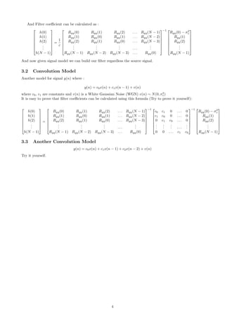
2. For l = 0
Rxy(0) = h(0)Ryy(0) + h(1)Ryy(1) + h(2)Ryy(2) + . . . + h(N − 1)Ryy(N − 1)
For l = 1
Rxy(1) = h(0)Ryy(−1) + h(1)Ryy(0) + h(2)Ryy(1) + . . . + h(N − 1)Ryy(N − 2)
and for WSS signal Ryy(−k) = Ryy(k) So
Rxy(1) = h(0)Ryy(1) + h(1)Ryy(0) + h(2)Ryy(1) + . . . + h(N − 1)Ryy(N − 2)
For l = N − 1
Rxy(N − 1) = h(0)Ryy(N − 1) + h(1)Ryy(N − 2) + . . . + h(N − 1)Ryy(0)
So in Matrix form







Rxy(0)
Rxy(1)
Rxy(2)
...
Rxy(N − 1)







=







Ryy(0) Ryy(1) Ryy(2) . . . Ryy(N − 1)
Ryy(1) Ryy(0) Ryy(1) . . . Ryy(N − 2)
Ryy(2) Ryy(1) Ryy(0) . . . Ryy(N − 3)
...
...
... . . .
...
Ryy(N − 1) Ryy(N − 2) Ryy(N − 3) . . . Ryy(0)














h(0)
h(1)
h(2)
...
h(N − 1)







To get filter coefficients







h(0)
h(1)
h(2)
...
h(N − 1)







=







Ryy(0) Ryy(1) Ryy(2) . . . Ryy(N − 1)
Ryy(1) Ryy(0) Ryy(1) . . . Ryy(N − 2)
Ryy(2) Ryy(1) Ryy(0) . . . Ryy(N − 3)
...
...
... . . .
...
Ryy(N − 1) Ryy(N − 2) Ryy(N − 3) . . . Ryy(0)







−1 






Rxy(0)
Rxy(1)
Rxy(2)
...
Rxy(N − 1)







2.1 Results of filtering
Figure 2 shows the results of applying a 4th order Wiener filter on a distorted sin signal with some smoothing.
The value of the mean square error MSE is extremely reduced from to 0.0036
3 Wiener filter using signal models
In the previous section we assumed that we already have the source signal x(n) which is not applicable in real
life. Actually we always have not this signal x(n). It makes sense as if we have it, so why to use Wiener filter
to estimate it. As we don’t have signal x(n), we can’t get Rxy and so we can’t build our filter. But we can get
Rxy in terms of Ryy if we can model signal y(n) as a function of signal x(n)
3.1 Linear Model
In this model we assume that signal y(n) is a linear transformation of signal x(n) i.e:
y(n) = cx(n) + v(n)
where c is a constant and v(n) is a White Gaussian Noise (WGN) v(n) ∼ N(0, σ2
v)
So
Ryy(0) = E[y(n)(cx(n) + v(n))]
Ryy(0) = cE[y(n)x(n)] + E[y(n)v(n))]
Ryy(0) = cRxy(0) + E[(cx(n) + v(n)v(n)]
Ryy(0) = cRxy(0) + cE[x(n)v(n)] + E[v(n)2
]
Ryy(0) = cRxy(0) + σ2
v
where E[x(n)v(n)] = 0 uncorrelated signals.
Similarly
2

3. Figure 2: Results of applying 4th order Wiener filter. MSE = 0.0036
Ryy(1) = E[y(n − 1)(cx(n) + v(n))]
Ryy(1) = cE[y(n − 1)x(n)] + E[y(n − 1)v(n))]
Ryy(1) = cRxy(1)
Ryy(2) = cRxy(2)
...
Ryy(N − 1) = cRxy(N − 1)
In matrix form







Rxy(0)
Rxy(1)
Rxy(2)
...
Rxy(N − 1)







= 1
c ×







Ryy(0) − σ2
Ryy(1)
Rxy(2)
...
Ryy(N − 1)







3

4. And Filter coefficient can be calculated as :







h(0)
h(1)
h(2)
...
h(N − 1)







=
1
c







Ryy(0) Ryy(1) Ryy(2) . . . Ryy(N − 1)
Ryy(1) Ryy(0) Ryy(1) . . . Ryy(N − 2)
Ryy(2) Ryy(1) Ryy(0) . . . Ryy(N − 3)
...
...
... . . .
...
Ryy(N − 1) Ryy(N − 2) Ryy(N − 3) . . . Ryy(0)







−1 






Ryy(0) − σ2
v
Ryy(1)
Ryy(2)
...
Ryy(N − 1)







And now given signal model we can build our filter regardless the source signal.
3.2 Convolution Model
Another model for signal y(n) where :
y(n) = c0x(n) + c1x(n − 1) + v(n)
where c0, c1 are constants and v(n) is a White Gaussian Noise (WGN) v(n) ∼ N(0, σ2
v)
It is easy to prove that filter coefficients can be calculated using this formula (Try to prove it yourself):







h(0)
h(1)
h(2)
...
h(N − 1)







=







Ryy(0) Ryy(1) Ryy(2) . . . Ryy(N − 1)
Ryy(1) Ryy(0) Ryy(1) . . . Ryy(N − 2)
Ryy(2) Ryy(1) Ryy(0) . . . Ryy(N − 3)
...
...
... . . .
...
Ryy(N − 1) Ryy(N − 2) Ryy(N − 3) . . . Ryy(0)







−1 






c0 c1 0 . . . 0
c1 c0 0 . . . 0
0 c1 c0 . . . 0
...
...
... . . .
...
0 0 . . . c1 c0







−1 






Ryy(0) − σ2
v
Ryy(1)
Ryy(2)
...
Ryy(N − 1)







3.3 Another Convolution Model
y(n) = c0x(n) + c1x(n − 1) + c2x(n − 2) + v(n)
Try it yourself.
4