Download to read offline
![Stochastic Section # 4
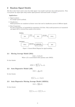
Random Signals & Random Signal Models
Eslam Adel
March 21, 2018
1 Random Signals
1. Random signal is a sequence of random variables [x1, x2, x3, . . . , xN ].
2. Mean of the random signal E[x] can be approximated as
E[x] =
1
N
N−1
i=0
xi (1)
3. Sample Autocorrelation Rxnxn+k
is defined as:
Rxnxn+k
=
1
N
N−1−k
i=0
xi+kxi k = 0, 1, 2, . . . N (2)
4. We always assume that the signal is zero mean. If the signal is not zero mean, subtract the mean from it.
x → x − E[x]
Note: for zero mean signal Rxx = σ2
5. For random signal it is assumed that it is a wide sense stationary signal (WSS) Where :
1. E[x] = constant
2. Rxn+kxn = E[xn+kxn] = Rxx(k) (not a function of time variable n)
6. Stationarity means that for different windows of the same signal, statistical parameters are almost the
same.
7. For WSS signal Rxx(k) = Rxx(−k)
1.1 Example
Assume signal x[n] = [1, 2, 3, 4, 5]
Evaluate the following:
1. Rxx(0)
2. Rxx(−1)
3. Rxx(1)
Solution :
At first make sure that signal is zero mean
m = 3 so x[n] will be
x[n] = [−2, −1, 0, 1, 2]
1](https://image.slidesharecdn.com/section4-200826012403/85/Section4-stochastic-1-320.jpg)
![Stochastic Section # 4
Random Signals & Random Signal Models
Eslam Adel
March 21, 2018
1 Random Signals
1. Random signal is a sequence of random variables [x1, x2, x3, . . . , xN ].
2. Mean of the random signal E[x] can be approximated as
E[x] =
1
N
N−1
i=0
xi (1)
3. Sample Autocorrelation Rxnxn+k
is defined as:
Rxnxn+k
=
1
N
N−1−k
i=0
xi+kxi k = 0, 1, 2, . . . N (2)
4. We always assume that the signal is zero mean. If the signal is not zero mean, subtract the mean from it.
x → x − E[x]
Note: for zero mean signal Rxx = σ2
5. For random signal it is assumed that it is a wide sense stationary signal (WSS) Where :
1. E[x] = constant
2. Rxn+kxn = E[xn+kxn] = Rxx(k) (not a function of time variable n)
6. Stationarity means that for different windows of the same signal, statistical parameters are almost the
same.
7. For WSS signal Rxx(k) = Rxx(−k)
1.1 Example
Assume signal x[n] = [1, 2, 3, 4, 5]
Evaluate the following:
1. Rxx(0)
2. Rxx(−1)
3. Rxx(1)
Solution :
At first make sure that signal is zero mean
m = 3 so x[n] will be
x[n] = [−2, −1, 0, 1, 2]
1](https://image.slidesharecdn.com/section4-200826012403/75/Section4-stochastic-1-2048.jpg)
![1. Rxx(0)
Rxx(0) = 1
5 [−2, −1, 0, 2, 1] × [−2, −1, 0, 1, 2] = 10
5 = 2
2. Rxx(1)
Rxx(1) = 1
5 [−2, −1, 0, 2, 1] × [0, −2, −1, 0, 1] = 4
5
3. Rxx(−1)
Rxx(−1) = 1
5 [−2, −1, 0, 2, 1] × [−1, 0, 1, 2, 0] = 4
5
Note:
For WSS signal Rxx(k) = Rxx(−k)
1.2 Problem 1.25
A random signal x(n) is defined as a linear function of time by
x(n) = an + b (3)
where a and b are independent zero-mean gaussian random variables of variances σ2
a and σ2
b , respectively.
1. Compute E[x(n)]2
.
2. Is x(n) a stationary process? Explain.
3. For each fixed n, compute the probability density p(x(n))
Solution :
1. E[x(n)]2
E[x(n)2
] = E[(an + b)2
] = E[a2
n2
+ 2anb + b2
]
E[x(n)2
] = n2
E[a2
] + E[b2
] + 2nE[ab]
E[a2
] = σ2
a − 0 = σ2
a,E[b2
] = σ2
b and E[ab] = E[a]E[b] = 0:
E[x(n)2
] = n2
σ2
a + σ2
b
2. To check a signal is WSS or not
1. E[x] = 0 = const So we have to check the correlation
2. Rxx
Rxn+kxn
= E[xn+kxn] = E[(a(n + k) + b)(an + b)] = n(n + k)E[a2
] + E[b2
]
Rxn+kxn
= n(n + k)σ2
a + σ2
b
Rxx(k) is a function in time variable So x(n) is not WSS
3. p(x(n))
x(n) = an + b where a ∼ N(0, σ2
a) and b ∼ N(0, σ2
b )
So x ∼ N(0, σ2
x) and σ2
x = E[x2
] − m2
x = n2
σ2
a + σ2
b
p(x(n)) = 1√
2πσx
e
−x2
2σ2
x
2](https://image.slidesharecdn.com/section4-200826012403/85/Section4-stochastic-2-320.jpg)
![Figure 2: Linear Estimation of signal
3 Linear Estimation of Signal
What’s beyond building signal model? We have to determine model parameters. But How to select them ?.
There is different ways to determine model parameters. Different methods are proposed. We will have two of
them.
So the case now is that we have a signal x that is changed due to noise to be another signal y. We applied
our model on y to estimate x so we got ˜x. see figure 2
3.1 Maximum Likelihood Method (ML)
The idea is to maximize the joint probability function of all random variables f(x1, x2, . . . , xN )
Applying this on first order autoregressive model AR(1)
X(Z) = 1
1−aZ−1 (Z)
model parameters are a and σ2
Solution will be :
a =
N−1
n=1 xnxn−1
N−1
n=1 x2
n−1
σ2
= 1
N
N−1
n=1 (x(n) − ax(n − 1))
3.2 Mean Square Error Method (MS)
Error is defined as :
e = x − ˜x
So the mean square error will be
E[(x − ˜x)2
]
to minimize the error differentiation of MSe with respect to model parameters must be zero.
Lets see an example:
3.2.1 Example 1
Assume
˜x = ay
Determine value of a that minimize the mean square error.
Solution:
MSe = E[e2
] = E[(x − ˜x)2
] = E[(x − ay)2
]
∂MSe
∂a = 0
E[2(x − ay) × −y] = 0
−E[xy] + aE[y2
] = 0
a = E[xy]
E[y2]
a =
Rxy(0)
Ryy(0)
5](https://image.slidesharecdn.com/section4-200826012403/85/Section4-stochastic-5-320.jpg)
![3.2.2 Example 2
Given
˜x = ay(n) + by(n − 1)
Determine values of a and b to minimize the mean square error.
Solution:
MSe = E[e2
] = E[(x − ˜x)2
] = E[(x − ayn − byn−1)2
]
∂MSe
∂a = 0
E[2(x − ayn − byn−1) × −yn] = 0
−E[xy] + aE[y2
] + bE[yn−1yn] = 0
aRyy(0) + bRyy(1) = Rxy(0) (4)
Similarly for b
∂MSe
∂b = 0
E[2(x − ayn − byn−1) × −yn−1] = 0
−E[xyn−1] + aE[y2
ny2
n−1] + bE[y2
n−1] = 0
aRyy(1) + bRyy(0) = Rxy(1) (5)
We can put it in matrix form
Ryy(0) Ryy(1)
Ryy(1) Ryy(0)
a
b
=
Rxy(0)
Rxy(1)
(6)
Finally
a
b
=
Ryy(0) Ryy(1)
Ryy(1) Ryy(0)
−1
Rxy(0)
Rxy(1)
(7)
6](https://image.slidesharecdn.com/section4-200826012403/85/Section4-stochastic-6-320.jpg)

1. The document discusses random signal models, which represent random signals using parameters from probability distributions rather than storing the entire signals. This allows generation, classification, and compression of random signals. 2. Common random signal models include the moving average (MA), autoregressive (AR), and autoregressive moving average (ARMA) models. The maximum likelihood and mean square error methods are presented for determining the model parameters that best represent a signal. 3. An example shows determining the parameters a and b for an ARMA(1,1) model that estimates a signal x from another signal y by minimizing the mean square error between x and the model output. The parameters are calculated from the autocorrelation and crosscorrelation