Download as PDF, PPTX
![The minimum enclosing ball problem [Tax and Duin, 2004]
Stéphane Canu (INSA Rouen - LITIS) May 12, 2014 3 / 35](https://image.slidesharecdn.com/lecture6svdd-140315083044-phpapp02/85/Lecture6-svdd-3-320.jpg)
![The minimum enclosing ball problem [Tax and Duin, 2004]
the center
Stéphane Canu (INSA Rouen - LITIS) May 12, 2014 3 / 35](https://image.slidesharecdn.com/lecture6svdd-140315083044-phpapp02/85/Lecture6-svdd-4-320.jpg)
![The minimum enclosing ball problem [Tax and Duin, 2004]
the radius
Given n points, {xi , i = 1, n} .
min
R∈IR,c∈IRd
R2
with xi − c 2
≤ R2
, i = 1, . . . , n
What is that in the convex programming hierarchy?
LP, QP, QCQP, SOCP and SDP
Stéphane Canu (INSA Rouen - LITIS) May 12, 2014 3 / 35](https://image.slidesharecdn.com/lecture6svdd-140315083044-phpapp02/85/Lecture6-svdd-5-320.jpg)


![MEB and the one class SVM
SVDD:
min
w,ρ
1
2 w 2
− ρ
with w xi ≥ ρ + 1
2 xi
2
SVDD and linear OCSVM (Supporting Hyperplane)
if ∀i = 1, n, xi
2
= constant, it is the the linear one class SVM (OC SVM)
The linear one class SVM [Schölkopf and Smola, 2002]
min
w,ρ
1
2 w 2
− ρ
with w xi ≥ ρ
with ρ = ρ + 1
2 xi
2
⇒ OC SVM is a particular case of SVDD
Stéphane Canu (INSA Rouen - LITIS) May 12, 2014 6 / 35](https://image.slidesharecdn.com/lecture6svdd-140315083044-phpapp02/85/Lecture6-svdd-8-320.jpg)


![Variations over SVDD
Adaptive SVDD: the weighted error case for given wi , i = 1, n
min
c∈IRp,R∈IR,ξ∈IRn
R + C
n
i=1
wi ξi
with xi − c 2
≤ R+ξi
ξi ≥ 0 i = 1, n
The dual of this problem is a QP [see for instance Liu et al., 2013]
min
α∈IRn
α XX α − α diag(XX )
with
n
i=1 αi = 1 0 ≤ αi ≤ Cwi i = 1, n
Density induced SVDD (D-SVDD):
min
c∈IRp,R∈IR,ξ∈IRn
R + C
n
i=1
ξi
with wi xi − c 2
≤ R+ξi
ξi ≥ 0 i = 1, n](https://image.slidesharecdn.com/lecture6svdd-140315083044-phpapp02/85/Lecture6-svdd-19-320.jpg)


![An important theoretical result
For a well-calibrated bandwidth,
The SVDD estimates the underlying distribution level set [Vert and Vert,
2006]
The level sets of a probability density function IP(x) are the set
Cp = {x ∈ IRd
| IP(x) ≥ p}
It is well estimated by the empirical minimum volume set
Vp = {x ∈ IRd
| k(x, .) − f (.) 2
H − R2
≥ 0}
The frontiers coincides](https://image.slidesharecdn.com/lecture6svdd-140315083044-phpapp02/85/Lecture6-svdd-25-320.jpg)
![SVDD: the generalization error
For a well-calibrated bandwidth,
(x1, . . . , xn) i.i.d. from some fixed but unknown IP(x)
Then [Shawe-Taylor and Cristianini, 2004] with probability at least 1 − δ,
(∀δ ∈]0, 1[), for any margin m > 0
IP k(x, .) − f (.) 2
H ≥ R2
+ m ≤
1
mn
n
i=1
ξi +
6R2
m
√
n
+ 3
ln(2/δ)
2n](https://image.slidesharecdn.com/lecture6svdd-140315083044-phpapp02/85/Lecture6-svdd-26-320.jpg)


![Small Sphere and Large Margin (SSLM) approach
Support vector data description with margin [Wu and Ye, 2009]
min
w,R,ξ∈IRn
R2
+C
yi =1
ξ+
i +
yi =−1
ξ−
i
with xi − c 2
≤ R2
− 1+ξ+
i , ξ+
i ≥ 0 i such that yi = 1
and xi − c 2
≥ R2
+ 1−ξ−
i , ξ−
i ≥ 0 i such that yi = −1
xi − c 2
≥ R2
+ 1−ξ−
i and yi = −1 ⇐⇒ yi xi − c 2
≤ yi R2
− 1+ξ−
i
L(c, R, ξ, α, β) = R2
+C
n
i=1
ξi +
n
i=1
αi yi xi − c 2
− yi R2
+ 1−ξi −
n
i=1
βi ξi
−4 −3 −2 −1 0 1 2 3
−3
−2
−1
0
1
2
3
4](https://image.slidesharecdn.com/lecture6svdd-140315083044-phpapp02/85/Lecture6-svdd-36-320.jpg)


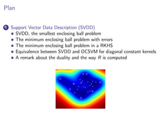
This document provides an overview of Support Vector Data Description (SVDD), which finds the minimum enclosing ball that encapsulates a set of data points. It discusses how SVDD can be formulated as a quadratic programming problem and outlines its dual formulation. The document also notes that SVDD generalizes to non-linear settings using kernels, and discusses variations like adaptive SVDD and density-induced SVDD. Key points covered include the representer theorem, KKT conditions, and how the radius of the enclosing ball can be determined from the Lagrangian.