Downloaded 43 times
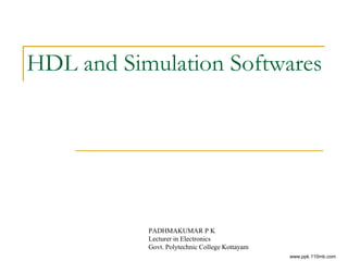
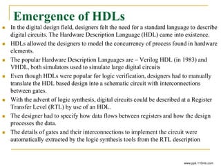
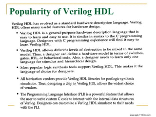
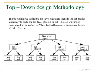
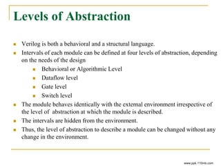
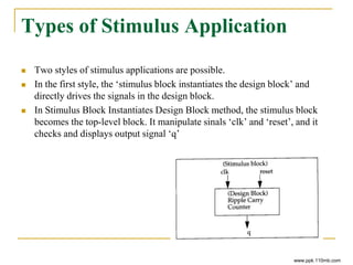
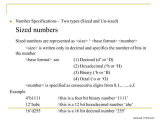
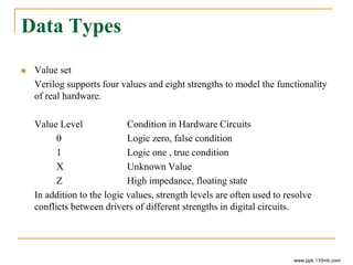
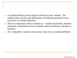
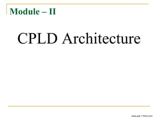
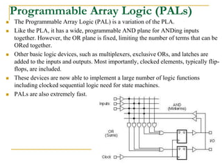
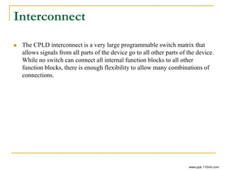
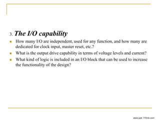
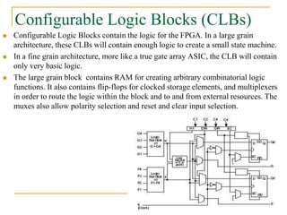
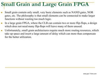
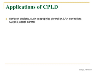
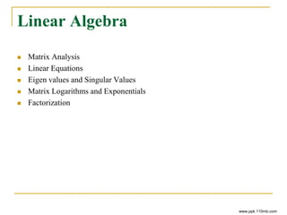
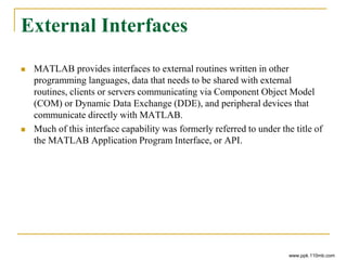
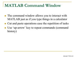
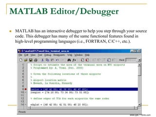
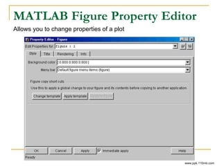
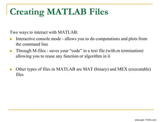
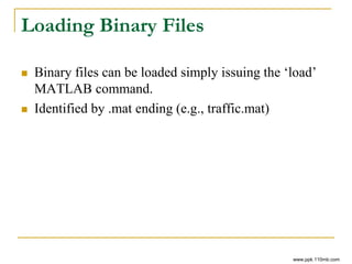
![Example – Ripple Carry Counter
Design Block
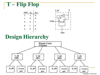
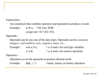
Let use top down design methodology
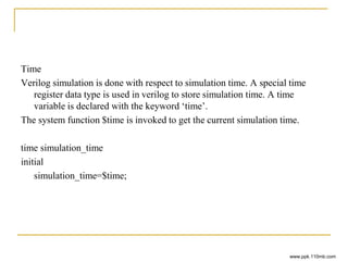
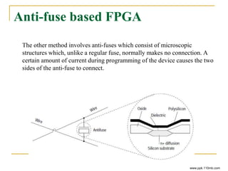
Verilog description of Ripple Carry Counter
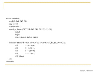
module ripple_carry_counter (q, clk, reset);
output [3:0] q;
input clk, reset;
T_FF tff0 (q[0], clk, reset);
T_FF tff1 (q[1], clk, reset);
T_FF tff2 (q[2], clk, reset);
T_FF tff3 (q[3], clk, reset);
endmodule
www.ppk.110mb.com](https://image.slidesharecdn.com/s6cad5-160127095854/85/S6-cad5-31-320.jpg)
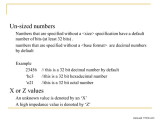
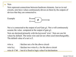
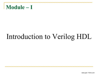
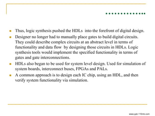
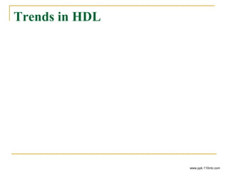
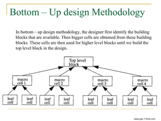
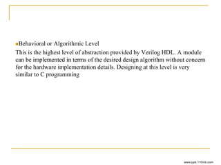
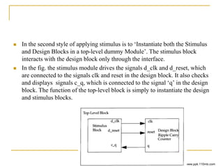
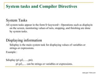
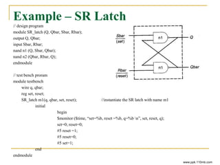
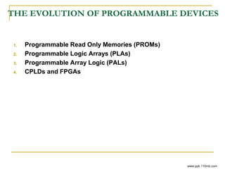
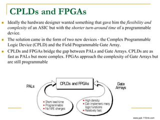
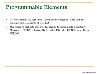
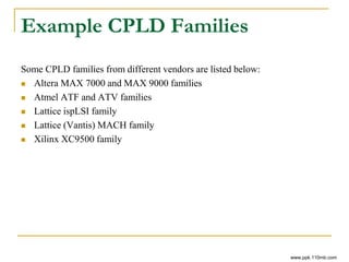
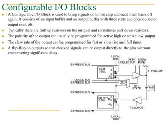
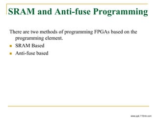
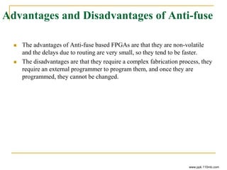
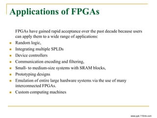
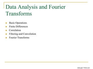
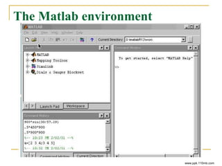
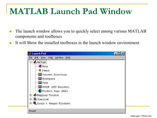
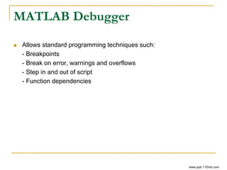
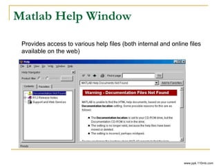
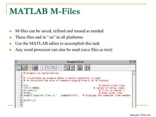
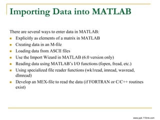
![Vectors
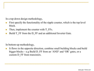
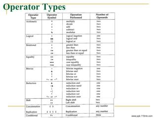
Nets or reg data types can be declared as vectors (multiple bit width). If bit
width is not specified, the default is scalar (1 bit)
Example
wire a; //scalar net variable
wire [7:0] bus; // 8-bit bus
wire [32:0] busA, busB, busC; //3 buses of 32 bit width
reg clock; //scalar register
reg [7:0] clock; // 8bit register
www.ppk.110mb.com](https://image.slidesharecdn.com/s6cad5-160127095854/85/S6-cad5-45-320.jpg)
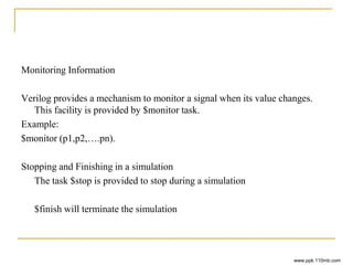
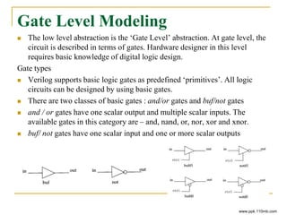

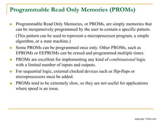
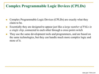
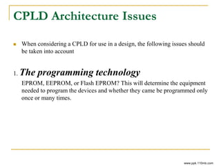
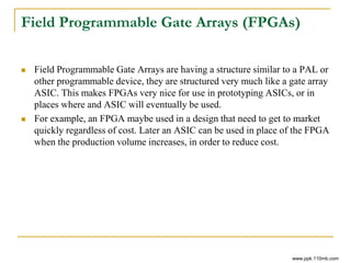
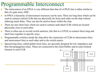
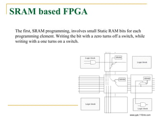
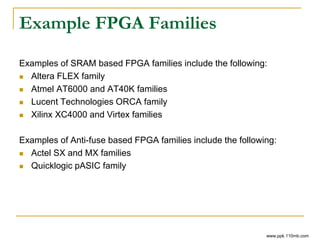
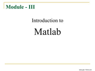
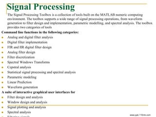
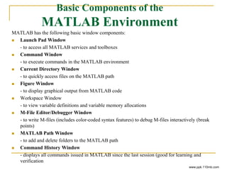
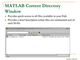
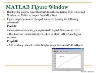
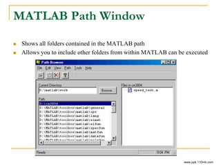
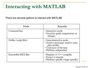
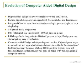
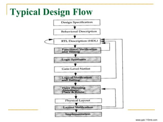
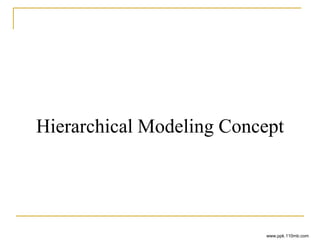
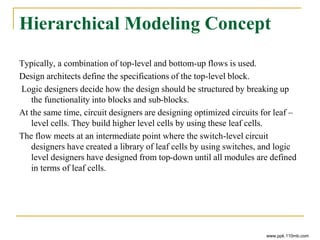
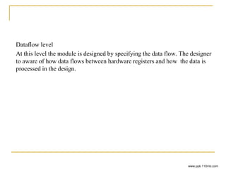
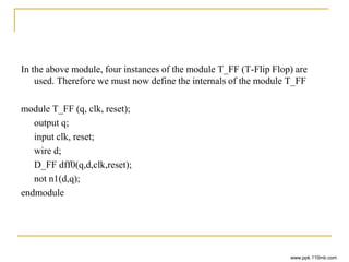
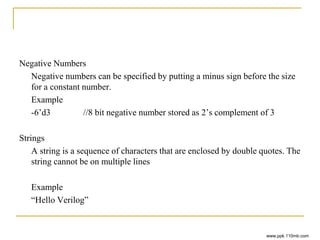
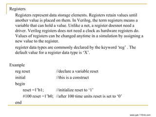
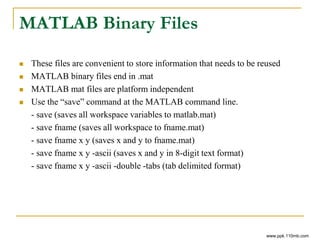
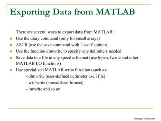
![Interactive Mode
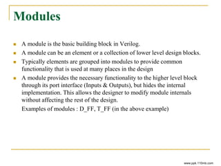
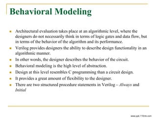
Use the MATLAB Command Window to interact with MATLAB in
“calculator” mode
>> a=[3 2 4; 4 5 6; 1 2 3]
Multiple commands can be executed using the semicolon “;” separator
between commands
>> a=[3 2 4; 4 5 6; 1 2 3] ; b=[3 2 5]’ ; c=a*b
This single line defines two matrices (a and b) and computes their product
(c)
Use the semi-colon “;” separator to tell the MATLAB to inhibit output to
the Command Window
Semi-colon is also used to differentiate between rows in a matrix definition
All commands can be executed within the MATLAB Command Window
www.ppk.110mb.com](https://image.slidesharecdn.com/s6cad5-160127095854/85/S6-cad5-121-320.jpg)
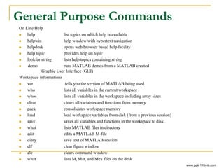
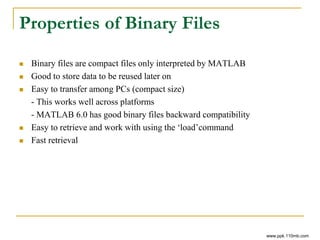
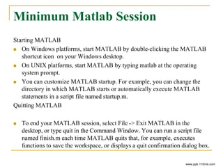
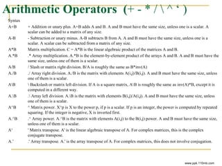
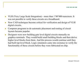
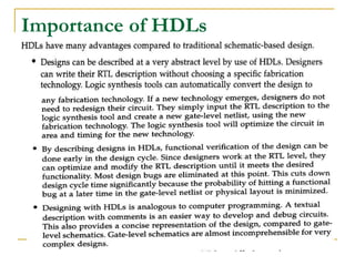
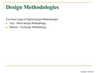
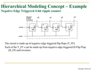
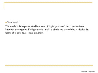
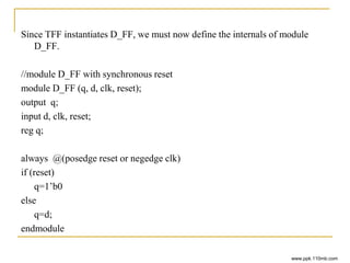
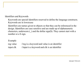
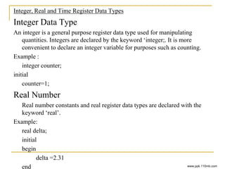
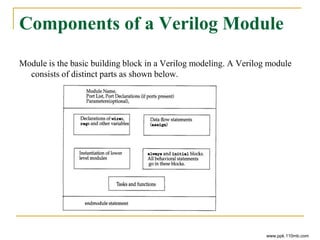
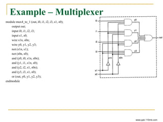
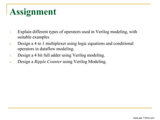
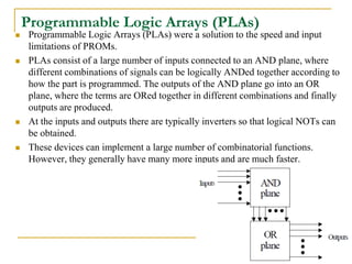
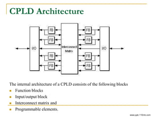
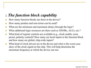
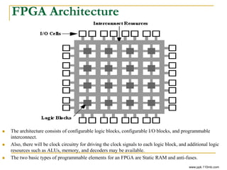
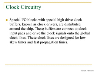
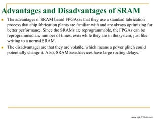
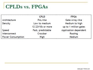
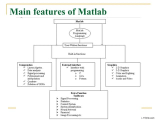
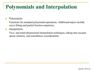
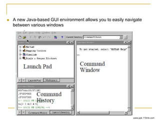
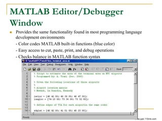
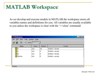
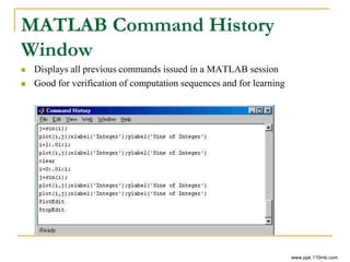
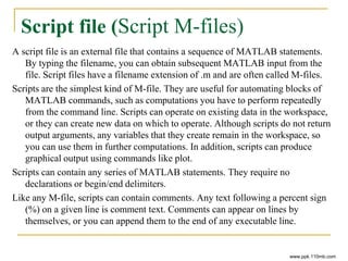
![Arrays (Array Operations)
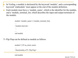
[ ] Array constructor
, Array row element separator
; Array column element separator
: Specify range of array elements
end Indicate last index of array
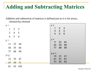
+ Addition or unary plus
- Subtraction or unary minus
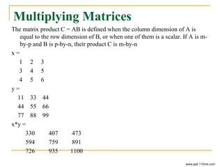
.* Array multiplication
./ Array right division
. Array left division
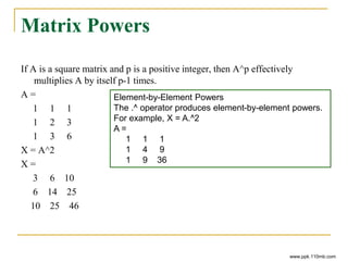
.^ Array power
.‘ Array (nonconjugated) transpose
www.ppk.110mb.com](https://image.slidesharecdn.com/s6cad5-160127095854/85/S6-cad5-137-320.jpg)
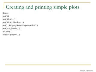
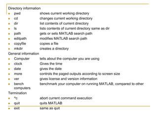
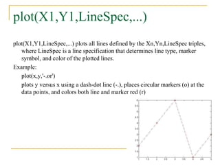
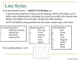
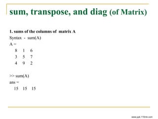
![plot(X1,Y1,...)
plot(X1,Y1,...) plots all lines defined by Xn versus Yn pairs. If only Xn or Yn
is a matrix, the vector is plotted versus the rows or columns of the matrix,
depending on whether the vector's row or column dimension matches the
matrix.
Example:
x=[1 2 3 4 5];
y=[2 4 6 1 3];
plot (x,y)
www.ppk.110mb.com](https://image.slidesharecdn.com/s6cad5-160127095854/85/S6-cad5-141-320.jpg)
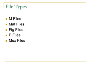
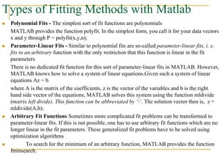
![sine plots
x=[0:0.25:2*pi];
y=sin(x);
plot(x,y);
x=[0:0.25:2*pi];
y=sin(x);
plot(x,y,’-.or’);
x=[0:0.25:2*pi];
y=sin(x);
stairs(x,y)
www.ppk.110mb.com](https://image.slidesharecdn.com/s6cad5-160127095854/85/S6-cad5-144-320.jpg)
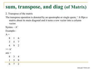
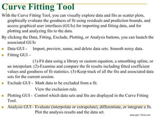
![Multiple data set in one graph
plot(x,y1,x,y2,x,y3)
>> x=[0:0.25:3*pi];
>> y1=sin(x);
>> y2=cos(x);
>> y3=tan(x);
>> plot(x,y1,x,y2,x,y3)
www.ppk.110mb.com](https://image.slidesharecdn.com/s6cad5-160127095854/85/S6-cad5-145-320.jpg)
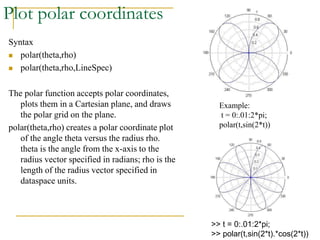
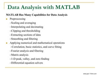
![scircle1
Compute coordinates of a small circle path from center, radius, and arc limits
Syntax
[latc,lonc] = scircle1(lat,lon,rng) returns the coordinates of points along small
circles centred at the points provided in lat and lon with radii given in rng.
These radii must in this case be given in the same angle units as the centre
points ('degrees').
Example:
[a,b]=scircle1(1,1,3);
plot(a,b)
www.ppk.110mb.com](https://image.slidesharecdn.com/s6cad5-160127095854/85/S6-cad5-147-320.jpg)
![scircle2
Compute coordinates of a small circle path from center and perimeter point
Syntax
[latc,lonc] = scircle2(lat1,lon1,lat2,lon2) returns the coordinates of points along
small circles centred at the points provided in lat1 and lon1, which pass
through the points provided in lat2 and lon2.
Example:
[a,b]=scircle2(1,1,3,3);
plot(a,b)
www.ppk.110mb.com](https://image.slidesharecdn.com/s6cad5-160127095854/85/S6-cad5-148-320.jpg)
![Function (Function M-files)
Syntax
function [out1, out2, ...] = funname(in1, in2, ...)
function [out1, out2, ...] = funname(in1, in2, ...) defines function funname that
accepts inputs in1, in2, etc. and returns outputs out1, out2, etc.
You add new functions to the MATLAB vocabulary by expressing them in terms
of existing functions. The existing commands and functions that compose the new
function reside in a text file called an M-file.
M-files can be either scripts or functions. Scripts are simply files containing a
sequence of MATLAB statements. Functions make use of their own local
variables and accept input arguments.
The name of an M-file begins with an alphabetic character and has a filename
extension of .m. The M-file name, less its extension, is what MATLAB searches
for when you try to use the script or function. A line at the top of a function M-file
contains the syntax definition. The name of a function, as defined in the first line
of the M-file, should be the same as the name of the file without the .m extension.
The variables within the body of the function are all local variables.
www.ppk.110mb.com](https://image.slidesharecdn.com/s6cad5-160127095854/85/S6-cad5-152-320.jpg)
![You can terminate any function with an end statement but, in most cases, this
is optional. end statements are required only in M-files that employ one or
more nested functions. Within such an M-file, every function (including
primary, nested, private, and subfunctions) must be terminated with an end
statement. You can terminate any function type with end, but doing so is
not required unless the M-file contains a nested function.
Functions normally return when the end of the function is reached. Use a
return statement to force an early return
Example :
function [mean,stdev] = stat(x)
n = length(x);
mean = sum(x)/n;
stdev = sqrt(sum((x-mean).^2/n));
end
www.ppk.110mb.com](https://image.slidesharecdn.com/s6cad5-160127095854/85/S6-cad5-153-320.jpg)
![Arrays and Matrices
Array Operations
[ ] Array constructor
, Array row element separator
; Array column element separator
: Specify range of array elements
end Indicate last index of array
+ Addition or unary plus
- Subtraction or unary minus
.* Array multiplication
./ Array right division
. Array left division
.^ Array power
.‘ Array (nonconjugated) transpose
www.ppk.110mb.com](https://image.slidesharecdn.com/s6cad5-160127095854/85/S6-cad5-154-320.jpg)
![Entering Matrices
We can enter matrices into MATLAB in several different ways:
Enter an explicit list of elements.
Load matrices from external data files.
Generate matrices using built-in functions.
Create matrices with your own functions in M-files
Separate the elements of a row with blanks or commas.
Use a semicolon ; to indicate the end of each row.
Surround the entire list of elements with square brackets, [ ]
A = [16 3 2 13; 5 10 11 8; 9 6 7 12; 4 15 14 1]
A =
16 3 2 13
5 10 11 8
9 6 7 12
4 15 14 1
www.ppk.110mb.com](https://image.slidesharecdn.com/s6cad5-160127095854/85/S6-cad5-155-320.jpg)
![Swap columns of a matrix
To swap columns of a matrix (rearrange the columns)
A =
16 2 3 13
5 11 10 8
9 7 6 12
4 14 15 1
>> B=A(:,[1 3 2 4])
B =
16 3 2 13
5 10 11 8
9 6 7 12
4 15 14 1
www.ppk.110mb.com](https://image.slidesharecdn.com/s6cad5-160127095854/85/S6-cad5-161-320.jpg)
![Concatenation
Concatenation is the process of joining small matrices to make bigger ones. In fact,
you made your first matrix by concatenating its individual elements. The pair of
square brackets, [], is the concatenation operator
A =
16 2 3 13
5 11 10 8
9 7 6 12
4 14 15 1
B =
16 3 2 13
5 10 11 8
9 6 7 12
4 15 14 1
>> [A B]
ans =
16 2 3 13 16 3 2 13
5 11 10 8 5 10 11 8
9 7 6 12 9 6 7 12
4 14 15 1 4 15 14 1
www.ppk.110mb.com](https://image.slidesharecdn.com/s6cad5-160127095854/85/S6-cad5-164-320.jpg)
![Deleting Rows and Columns
You can delete rows and columns from a matrix using just a pair of square
brackets
A =
16 3 13
5 10 8
9 6 12
4 15 1
>> A(:,2)=[]
A =
16 13
5 8
9 12
4 1
www.ppk.110mb.com](https://image.slidesharecdn.com/s6cad5-160127095854/85/S6-cad5-165-320.jpg)
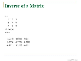
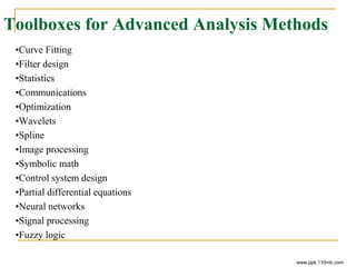
![Eigenvalues
An eigenvalue and eigenvector of a square matrix A are a scalar λ and a nonzero
vector v that satisfy,
Av= λv
p =
1 2 3
4 5 6
7 8 9
>> [v,d]=eig(p)
v =
-0.2320 -0.7858 0.4082
-0.5253 -0.0868 -0.8165
-0.8187 0.6123 0.4082
d =
16.1168 0 0
0 -1.1168 0
0 0 -0.0000 www.ppk.110mb.com](https://image.slidesharecdn.com/s6cad5-160127095854/85/S6-cad5-170-320.jpg)
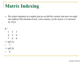
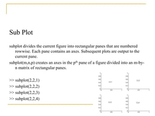
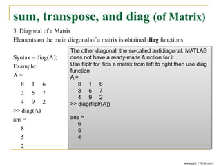
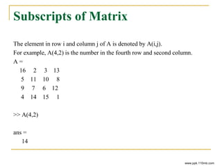
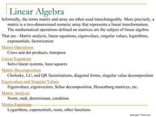
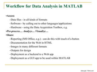
![Sub Matrix
The colon operator can also be used to pick out a certain row or column.
For example, the statement A(m:n,k:l) specifies rows m to n and column k
to l. Subscript expressions refer to portions of a matrix.
P =
1 3 4
5 4 3
5 6 7
>> P(2,:)
=
5 4 3
www.ppk.110mb.com
P =
1 3 4
5 4 3
5 6 7
>> P(:,2:3)
=
3 4
4 3
6 7
Creating a sub Matrix
P =
1 3 4
5 4 3
5 6 7
>> Q = P([2 3],[1 2])
Q =
5 4
5 6](https://image.slidesharecdn.com/s6cad5-160127095854/85/S6-cad5-173-320.jpg)


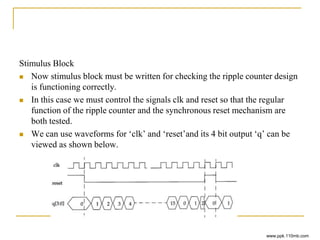
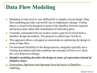
This document discusses the evolution of digital circuit design and computer-aided design techniques. It describes how hardware description languages (HDLs) like Verilog emerged to allow designers to model digital circuits at different levels of abstraction. HDLs enabled logic synthesis which automated the translation from register transfer level designs to gate-level implementations. The document outlines typical design flows involving hierarchical modeling and top-down or bottom-up methodologies. It also covers key concepts in HDLs like modules, instances, and different levels of abstraction for module implementation. Finally, it discusses the components of a simulation including separate stimulus and design blocks.