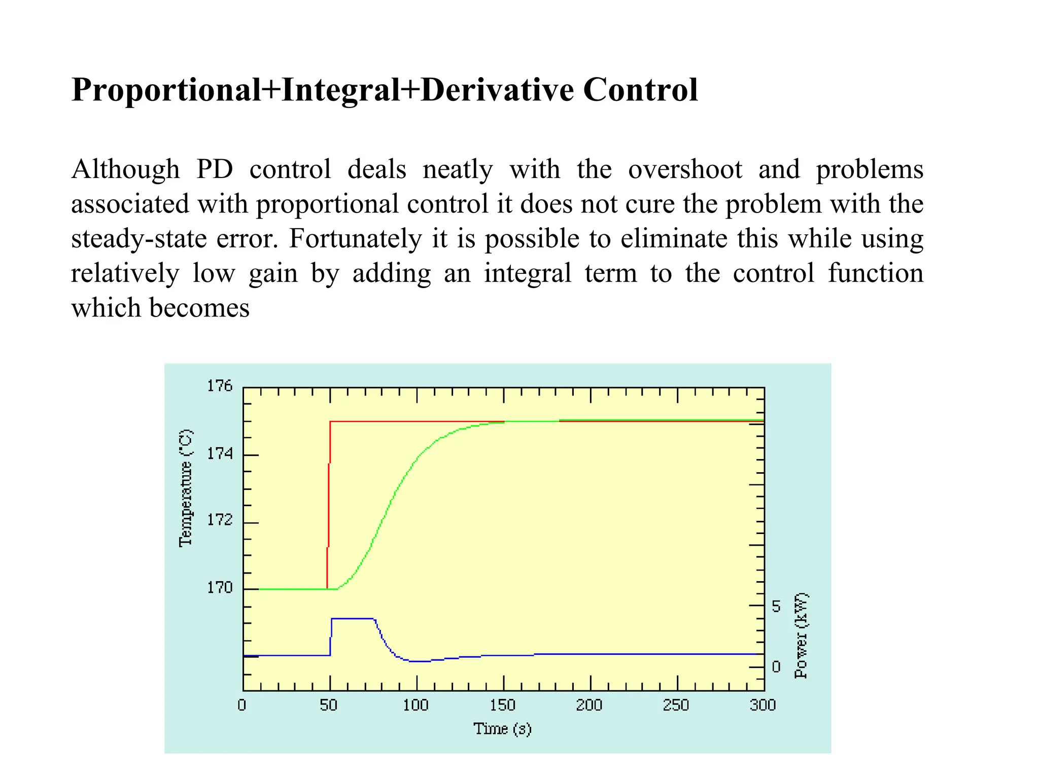
The document discusses various types of control in PID (Proportional-Integral-Derivative) systems, explaining how proportional control reduces rise time but can lead to steady-state errors, while derivative control mitigates overshoot and settling time. It outlines the significance of combining proportional, integral, and derivative controls for optimized system response and stability, and provides MATLAB examples for implementation. Additionally, it covers the design of lead and lag compensators through root locus techniques to adjust system stability and response speed.

1. PID Controller

2. Different Types of Feedback Control
On-Off Control
This is the simplest form of control.

3. Proportional Control
A proportional controller attempts to perform better than the On-off type by
applying power in proportion to the difference in temperature between the
measured and the set-point. As the gain is increased the system responds faster to
changes in set-point but becomes progressively underdamped and eventually
unstable. The final temperature lies below the set-point for this system because
some difference is required to keep the heater supplying power.

4. Proportional, Derivative Control
The stability and overshoot problems that arise when a proportional
controller is used at high gain can be mitigated by adding a term proportional
to the time-derivative of the error signal. The value of the damping can be
adjusted to achieve a critically damped response.

5. Proportional+Integral+Derivative Control
Although PD control deals neatly with the overshoot and problems
associated with proportional control it does not cure the problem with the
steady-state error. Fortunately it is possible to eliminate this while using
relatively low gain by adding an integral term to the control function
which becomes

6. The Characteristics of P, I, and D controllers
A proportional controller (Kp) will have the effect of reducing the
rise time and will reduce, but never eliminate, the steady-state
error.
An integral control (Ki) will have the effect of eliminating the
steady-state error, but it may make the transient response worse.
A derivative control (Kd) will have the effect of increasing the
stability of the system, reducing the overshoot, and improving the
transient response.

7. Proportional Control
By only employing proportional control, a steady state error
occurs.
Proportional and Integral Control
The response becomes more oscillatory and needs longer to
settle, the error disappears.
Proportional, Integral and Derivative Control
All design specifications can be reached.

8. CL RESPONSE RISE TIME OVERSHOOT SETTLING TIME S-S ERROR
Kp Decrease Increase Small Change Decrease
Ki Decrease Increase Increase Eliminate
Kd Small Change Decrease Decrease Small Change
The Characteristics of P, I, and D controllers

9. Tips for Designing a PID Controller
1. Obtain an open-loop response and determine what needs to be improved
2. Add a proportional control to improve the rise time
3. Add a derivative control to improve the overshoot
4. Add an integral control to eliminate the steady-state error
5. Adjust each of Kp, Ki, and Kd until you obtain a desired overall
response.
Lastly, please keep in mind that you do not need to implement all three
controllers (proportional, derivative, and integral) into a single system, if not
necessary. For example, if a PI controller gives a good enough response (like the
above example), then you don't need to implement derivative controller to the
system. Keep the controller as simple as possible.

10. num=1;
den=[1 10 20];
step(num,den)
Open-Loop Control - Example
G s
( )
1
s
2
10s
 20


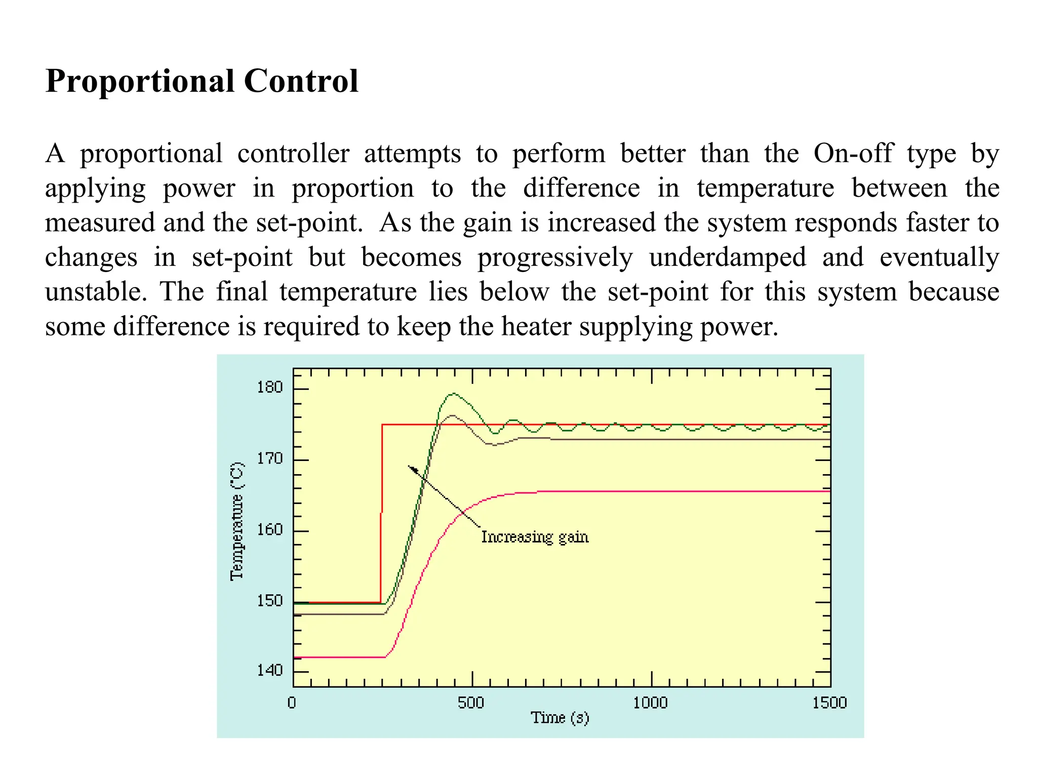
11. Proportional Control - Example
The proportional controller (Kp) reduces the rise time, increases
the overshoot, and reduces the steady-state error.
MATLAB Example
Kp=300;
num=[Kp];
den=[1 10 20+Kp];
t=0:0.01:2;
step(num,den,t)
Time (sec.)
Amplitude
Step Response
0 0.2 0.4 0.6 0.8 1 1.2 1.4 1.6 1.8 2
0
0.2
0.4
0.6
0.8
1
1.2
1.4
From: U(1)
To:
Y(1)
T s
( )
Kp
s
2
10 s

 20 Kp

( )

Time (sec.)
Amplitude
Step Response
0 0.2 0.4 0.6 0.8 1 1.2 1.4 1.6 1.8 2
0
0.1
0.2
0.3
0.4
0.5
0.6
0.7
0.8
0.9
1
From: U(1)
To:
Y(1)
K=300 K=100

12. Time (sec.)
Amplitude
Step Response
0 0.2 0.4 0.6 0.8 1 1.2 1.4 1.6 1.8 2
0
0.2
0.4
0.6
0.8
1
1.2
1.4
From: U(1)
To:
Y(1)
Kp=300;
Kd=10;
num=[Kd Kp];
den=[1 10+Kd 20+Kp];
t=0:0.01:2;
step(num,den,t)
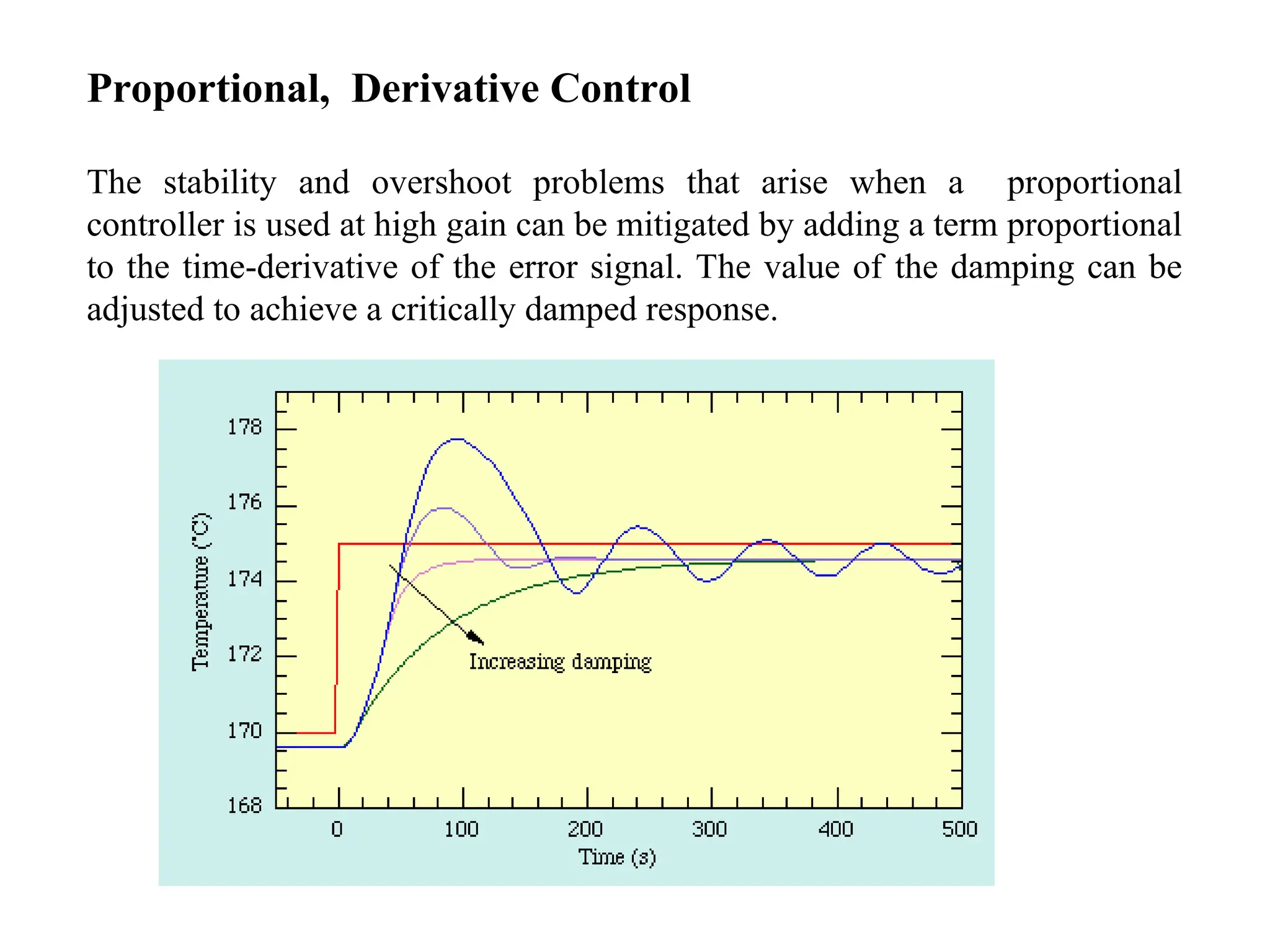
Proportional - Derivative - Example
The derivative controller (Kd) reduces both the overshoot and the
settling time.
MATLAB Example T s
( )
Kd s
 Kp

s
2
10 Kd

( ) s

 20 Kp

( )

Time (sec.)
Amplitude
Step Response
0 0.2 0.4 0.6 0.8 1 1.2 1.4 1.6 1.8 2
0
0.1
0.2
0.3
0.4
0.5
0.6
0.7
0.8
0.9
1
From: U(1)
To:
Y(1)
Kd=10
Kd=20

13. Proportional - Integral - Example
The integral controller (Ki) decreases the rise time, increases both
the overshoot and the settling time, and eliminates the steady-state
error
MATLAB Example
Time (sec.)
Amplitude
Step Response
0 0.2 0.4 0.6 0.8 1 1.2 1.4 1.6 1.8 2
0
0.2
0.4
0.6
0.8
1
1.2
1.4
From: U(1)
To:
Y(1)
Kp=30;
Ki=70;
num=[Kp Ki];
den=[1 10 20+Kp Ki];
t=0:0.01:2;
step(num,den,t)
T s
( )
Kp s
 Ki

s
3
10 s
2

 20 Kp

( ) s

 Ki

Time (sec.)
A
m
plitude
Step Response
0 0.2 0.4 0.6 0.8 1 1.2 1.4 1.6 1.8 2
0
0.2
0.4
0.6
0.8
1
1.2
1.4
From: U(1)
To:
Y(1)
Ki=70
Ki=100

14. Consider the following configuration:
Example - Practice

15. Lead or Phase-Lead Compensator Using Root Locus
A first-order lead compensator can be designed using the root locus. A lead compensator
in root locus form is given by
where the magnitude of z is less than the magnitude of p. A phase-lead compensator
tends to shift the root locus toward the left half plane. This results in an improvement in
the system's stability and an increase in the response speed.
When a lead compensator is added to a system, the value of this intersection will be a
larger negative number than it was before. The net number of zeros and poles will be the
same (one zero and one pole are added), but the added pole is a larger negative number
than the added zero. Thus, the result of a lead compensator is that the asymptotes'
intersection is moved further into the left half plane, and the entire root locus will be
shifted to the left. This can increase the region of stability as well as the response speed.
Gc s
( )
s z

( )
s p

( )

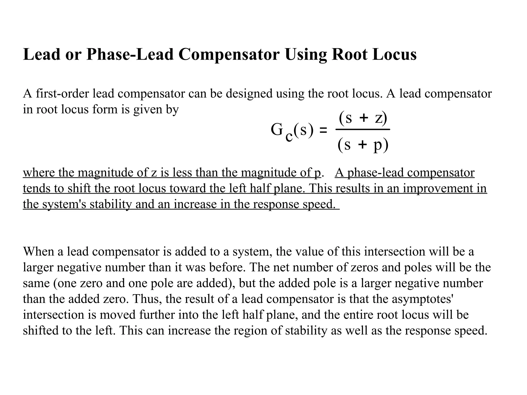
16. In Matlab a phase lead compensator in root
locus form is implemented by using the transfer
function in the form
numlead=kc*[1 z];
denlead=[1 p];
and using the conv() function to implement it
with the numerator and denominator of the plant
newnum=conv(num,numlead);
newden=conv(den,denlead);
Lead or Phase-Lead Compensator Using Root Locus

17. Lag or Phase-Lag Compensator Using Root Locus
A first-order lag compensator can be designed using the root locus. A lag compensator in root
locus form is given by
where the magnitude of z is greater than the magnitude of p. A phase-lag compensator tends to
shift the root locus to the right, which is undesirable. For this reason, the pole and zero of a lag
compensator must be placed close together (usually near the origin) so they do not appreciably
change the transient response or stability characteristics of the system.
When a lag compensator is added to a system, the value of this intersection will be a smaller
negative number than it was before. The net number of zeros and poles will be the same (one
zero and one pole are added), but the added pole is a smaller negative number than the added
zero. Thus, the result of a lag compensator is that the asymptotes' intersection is moved closer
to the right half plane, and the entire root locus will be shifted to the right.
Gc s
( )
s z

( )
s p

( )