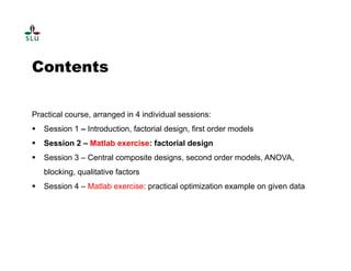
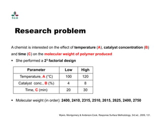
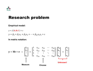
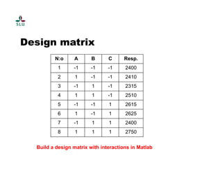
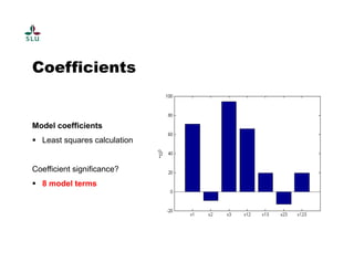
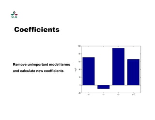
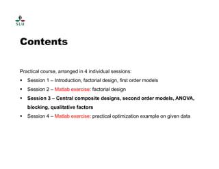
The document outlines a practical course on process and product optimization using design of experiments and response surface methodology, structured into four sessions covering factorial design, MATLAB exercises, and model analysis. It emphasizes the importance of design matrices, coefficients, residual analysis, ANOVA, and response contours in optimizing chemical processes. A specific research problem involving the effect of temperature, catalyst concentration, and time on polymer molecular weight is presented as a case study.

1. Process/product optimization
using design of experiments and
response surface methodology
M. Mäkelä
Sveriges landbruksuniversitet
Swedish University of Agricultural Sciences
Department of Forest Biomaterials and Technology
Division of Biomass Technology and Chemistry
Umeå, Sweden

2. Contents
Practical course, arranged in 4 individual sessions:
 Session 1 – Introduction, factorial design, first order models
 Session 2 – Matlab exercise: factorial design
 Session 3 – Central composite designs, second order models, ANOVA,
blocking, qualitative factors
 Session 4 – Matlab exercise: practical optimization example on given data

3. Session 1
Introduction
 Why experimental design
Factorial design
 Design matrix
 Model equation = coefficients
 Residual
 Response contour

4. Session 2
Factorial design
 Research problem
 Design matrix
 Model equation = coefficients
 Degrees of freedom
 Predicted response
 Residual
 ANOVA
 R2
 Response contour

5. Research problem
A chemist is interested on the effect of temperature (A), catalyst concentration (B)
and time (C) on the molecular weight of polymer produced
 She performed a 23 factorial design
Parameter Low High
Temperature, A (°C) 100 120
Catalyst conc., B (%) 4 8
Time, C (min) 20 30
 Molecular weight (in order): 2400, 2410, 2315, 2510, 2615, 2625, 2400, 2750
Myers, Montgomery & Anderson-Cook, Response Surface Methodology, 3rd ed., 2009, 131.

6. Research problem
Empirical model:
ݕ ൌ ݂ ۯ, ۰, ۱ ൅ ߝ
ݕ ൌ ߚ଴ ൅ ߚଵݔଵ ൅ ߚଶݔଶ ൅ ⋯ ൅ ߚ௞௝ݔ௞ݔ௝ ൅ ߝ
In matrix notation:
ܡ ൌ ܆܊ ൅ ܍ →
yଵ
yଶ
⋮
y୬
ൌ
1 ݔଵଵ ݔଶଵ ⋯ ݔଵ௞
1 ݔଵଶ ݔଶଶ ⋯ ݔଶ௞
1 ⋮ ⋮ ⋱ ⋮
1 ݔଵ௡ ݔଶ௡ ⋯ ݔ௡௞
b଴
bଵ
⋮
b୩
൅
eଵ
eଶ
⋮
e୬
Measure Choose
Unknown!

7. Design matrix
N:o A B C Resp.
1 -1 -1 -1 2400
2 1 -1 -1 2410
3 -1 1 -1 2315
4 1 1 -1 2510
5 -1 -1 1 2615
6 1 -1 1 2625
7 -1 1 1 2400
8 1 1 1 2750
Build a design matrix with interactions in Matlab

8. Coefficients
Model coefficients
 Least squares calculation
Coefficient significance?
 8 model terms

9. Degrees of freedom
In statistics, degrees of freedom (df) are lost by imposing linear constraints on
a sample
 E.g. sample variance:
ݏଶ ൌ Σ ሺ௬ି௬ത೔ ೙ ሻమ
೔సభ
௡ିଵ
where Σ ݕ െ ݕത ൌ 0. Hence ݊ െ 1 residuals can be used to completely
determine the other.
In RSM, dfs are lost due to the constraints imposed by the coefficients
 Residual df ݊ െ ݌ with ݊ observations and ݌ ൌ ݇ ൅ 1 model terms

10. Coefficients
Remove unimportant model terms
and calculate new coefficients

11. Predicted response
Calculate predicted response, ࢟ෝ
 Based on X and b
Graphical tools are useful

12. Residuals
Calculate model residuals
A common way is to scale the residuals
 E.g. standardized residual
→ Need an error approximation

13. Error estimation
Estimated error of predicted response
ߪොଶ ൌ Σ ሺ௬೔ି௬ො೔ሻమ
௡
௜ୀଵ , where p = k + 1
௡ି௣
Standardized residuals
 >│3│ a potential outlier

14. ANOVA
Analysis of variance (ANOVA) allows to statistically test the model
 Fisher’s F test
 H0: ߚ଴ ൌ ߚଵ ൌ ⋯ ൌ ߚ௞ ൌ 0
 H1: ߚ௝ ് 0 for at least one j
Parameter df Sum of
squares (SS)
Mean
square (MS)
F-value p-value
Total corrected n-1 SStot MStot
Regression k SSmod MSmod MSmod
/MSres
<0.05
>0.05
Residual n-k-1 SSres MSres
Lack of fit
Pure error

15. R2 statistic
ݕො௜
ݕ௜
݁௜
Data variability explained by the
model
 Compares model and total sum of
squares
R2 = 95.2%

16. Response contour
For a k=3 design, 2D contours require
one constant factor

17. Response contour
Use of the model
 Optimization within specific coordinates
 Prediction of an optimum
 Verification
A = 115 and B = 7
 ܠܕ ൌ ሾ1 .5 .5 1 .25ሿ
 ݕො௠ ൌ 2645 േ 90

18. Research problem
The chemist has a possibility to perform three
additional center-points in her factorial design
 Molecular weight values: 2800, 2750, 2810
Can this change our view on the behaviour of
the system?
A
B
C

19. Session 2
Factorial design
 Research problem
 Design matrix
 Model equation = coefficients
 Degrees of freedom
 Predicted response
 Residual
 ANOVA
 R2
 Response contour

20. Nomenclature
Design matrix
Coefficient
Degree of freedom
Prediction
Residual
Outlier
ANOVA
Sum of squares
Mean square
Contour

21. Contents
Practical course, arranged in 4 individual sessions:
 Session 1 – Introduction, factorial design, first order models
 Session 2 – Matlab exercise: factorial design
 Session 3 – Central composite designs, second order models, ANOVA,
blocking, qualitative factors
 Session 4 – Matlab exercise: practical optimization example on given data

22. Thank you for listening!